Many DSP algorithms are designed to target frequencies within a given signal. This makes it essential to be able to view the frequency response of an algorithm, and is why I had to bring in an external tool to view the results of the low- and high-pass filters in the previous project log.

DSP PAW aims to be an all-in-one solution, and so I set aside some time to implement the ability to view the frequencies present in the output signal. The previous log used spectrograms, which show magnitude over a range of frequencies over a range of time. A simpler approach would be to drop the range of time, only showing the instantaneous frequency magnitudes; this is possible by implementing the Fourier transform.

For computer applications, the Fourier transform can be efficiently calculated through what is known as the "Fast Fourier Transform" (FFT). Instead of "reinventing" the wheel, I chose a C library called kissfft to take care of the FFT calculations.

Designing the FFT visualization

The GUI uses the imgui framework to build its interface, making the addition of this feature fairly simple. To start, a checkbox is added to the menu which controls a drawFrequencies flag that will be used to make the visualizer visible:

bool drawFrequencies = false;
// ...
ImGui::Checkbox("Plot over freq.", &drawFrequencies); 

Later on in the rendering code, we simply add an if-statement that checks the drawFrequencies flag and renders the visualizer if true. This is the exact approach taken for the current signal plotter; in fact, most of the current plotter's code will be copied for this new visualization. The only significant difference will be the application of the FFT to the data before plotting.

The first FFT change is within a conditional that checks for changes in the sample buffer size. This prepares our buffers for taking in the incoming samples, as well as the kissfft configuration structure which needs to know this buffer size.

// Adds new samples to bufferCirc unless the block size has changed.
auto newSize = pullFromDrawQueue(bufferCirc);

if (newSize > 0) {
    // Sample block size has changed, resize buffers.
    buffer.resize(newSize);
    bufferFFTIn.resize(newSize);
    bufferFFTOut.resize(newSize);
    bufferCirc = CircularBuffer(buffer);
    pullFromDrawQueue(bufferCirc);

    // FFT: Re-initialize kissfft's configuration.
    kiss_fftr_free(kisscfg);
    kisscfg = kiss_fftr_alloc(buffer.size(), false, nullptr, nullptr);
}

kissfft needs separate input and output buffers (bufferFFTIn and bufferFFTOut) due to type differences: our samples come in as 16-bit unsigned integers, the FFT calculation requires floating-point values, and the calculation results are complex numbers.

So, we use std::copy to move the raw samples into bufferFFTIn, and then call kiss_fftr to perform a "real" FFT since we don't care about the imaginary components of the calculation.

std::copy(buffer.begin(), buffer.end(), bufferFFTIn.begin());
kiss_fftr(kisscfg, bufferFFTIn.data(), bufferFFTOut.data());

// Plot real values only: bufferFFTOut[i].r

When building the plot, the x-axis will simply span the range of bufferFFTOut. The y-axis ends up being more difficult to put constraints on: to my knowledge there isn't a real unit (it's simply "magnitude"), and there isn't a clear upper bound either. Dividing the output by the sampling rate isn't enough, neither is taking a fourth of that division. However, this constrains the plot enough that we can observe spikes in present frequencies and make relative comparisons between them.

Testing the FFT visualizer

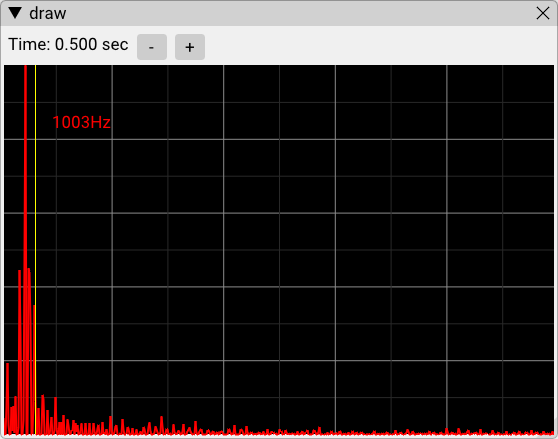
I tested this new feature by using the signal generator as an input signal with the default pass-through algorithm. This is the output given the input equation "0.8*sin(x/7)":

Given sampling rate Fs, an Fout frequency sine wave can be created with the equation sin(2*pi*x/Fs*Fout). At the default sampling rate of 32kHz, this means sin(x/7) creates a sine wave at about 728Hz. This would be the red spike in the above plot; the mouse cursor is controlling the yellow line, simply confirming that the frequency spike is a bit under 1kHz.

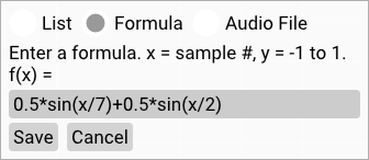
Now, we can write a new signal generator formula which adds a second sinusoidal component:

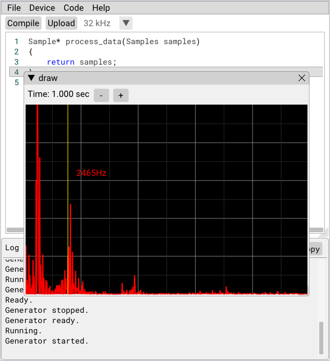
sin(x/2) would have a frequency of 2,546Hz following the Fs/Fout equation. With the new visualizer, we can confirm this is true:

While basic, this visualizer gives the GUI a great boost in analysis capabilities. More can certainly be done here, from quantifying the y-axis to layering the input frequency response to plotting maximums or averages for steadier output. For now, I'll leave this as-is and get back to finishing up the new hardware design...

Realizing the hardware and software for DSP PAW is central to the project's success; however, examples of algorithm implementations will be essential for making DSP PAW an adaptable solution. So, I've begun work on some guides that walk through writing and analyzing some common algorithms. As they're finished, these guides will get uploaded or linked to the project's code repository. Below is a kind of "rough draft" of what I would include in a guide; in the future, I will most likely post about newly available guides rather than writing them in these logs.

In short, both the low- and high-pass filters follow this formula:

y[n] = b0 * x[n] + b1 * x[n - 1] - a1 * y[n - 1]

...which is conveniently already valid C++ code. The coefficients a1, b0, and b1 can be calculated into variables given specified cut-off (Fc) and sampling (Fs) frequencies:

constexpr float Fc = 1000;
constexpr float Fs = 32000;


constexpr float Omega = 2 * 3.14159f * Fc / Fs;
constexpr float K = tan(Omega / 2.f);
constexpr float alpha = 1 + K;

constexpr float a1 = -(1 - K) / alpha;

// For low-pass filtering:
constexpr float b0 = K / alpha;
constexpr float b1 = b0;

// For high-pass:
constexpr float b0 = 1 / alpha;
constexpr float b1 = -b0;

By using the constexpr keyword, these values are calculated at compile-time, reducing execution time. Unfortunately, the above code will have an issue with the current DSP PAW software: a custom tan() implementation that calls into the core firmware will prevent K's compile-time evaluation. This can be fixed, but for now K will need to be calculated by hand and typed in.

One more requirement of these filters is that the sample data needs to be centered at zero. So, a short "normalization" function is written to convert a sample's 0 through 4095 integer value into a decimal -1.0 to 1.0 range. It may be possible to integrate this transformation into the filter as a performance optimization.

inline float N(Sample s) {
    return (s - 2048) / 2048.f;
}

Finally, we write the iterative loop that calculates each output sample. A buffer is defined to store the output since the input samples need to be preserved for calculation. If that were not the case, the sample buffer passed into process_data could be reused:

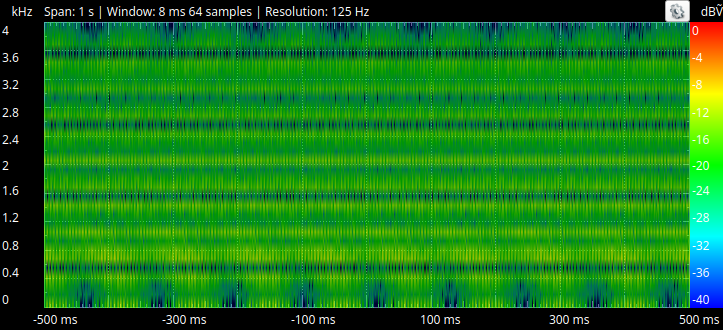
Sample* process_data(Samples x) {
	static Samples y;

	for (int n = 1; n < SIZE; ++n) {
		float y_n = b0 * N(x[n]) + b1 * N(x[n - 1]) - a1 * N(y[n - 1]);
		y[n] = (y_n + 1.f) * 2048; // return to 0-4095 range
	}

	return y;
}

To test these filters, I used an Analog Discovery 2. The software for this device is advanced, and provided me with a sweeped-frequency signal and a spectrogram to capture the filters' frequency responses. Both of these features could (and should) be built into DSP PAW. For now, testing without external hardware could have been done by loading the on-board signal generator with a sine wave (or perhaps low- and high-frequency sine waves added together) and observing the output's attenuation/form through the signal visualizer.

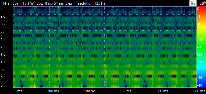
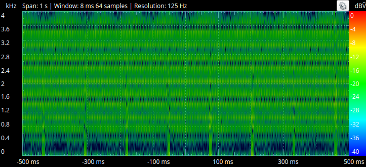
Here is the spectrogram with no filter running. All frequencies in the sweep are showing up in green:

With the implemented low-pass filter, attenuation of frequencies higher than 1kHz can be seen. Due to the nature of first-order IIR filtering, the attenuation is gradual and not "strong" at the specified cut-off.

The implemented high-pass filter passes through the frequencies beyond 1kHz, with attenuation below 1kHz clearly observable. Again, the cut-off's strength and spread is fairly weak.

As an extension to this algorithm, it is possible to control the targeted cut-off frequency at run-time with one of the add-on board's knobs. This is done by defining the alpha parameter as a function of the knob's position. For low-pass, the resulting alpha must be greater than 1, while for high-pass it needs to be less than 1. The K parameter must then be redefined in terms of alpha:

float alpha = param1() / 2047.f + 1.01f; // Low-pass: 1 < alpha <= 3
float K = alpha - 1.f; 

(One could also apply these filters to an audio signal -- the effect will be noticeable in recordings that include significant treble and/or bass.)

Many lines of development boards, especially the NUCLEO line from STMicroelectronics, have seen supply shortages over the past few years. This is a significant problem for DSP PAW since it currently only supports one (popular) NUCLEO variant.

Fortunately, this variant is in stock with distributors at the moment; though some are limiting purchase quantities. To avoid this issue, DSP PAW has two options:

1. Expand support for more NUCLEO boards.
2. Integrate an STM32 microcontroller into the "add-on" board to create a single, complete device.

Integration has been on the table ever since this project's inception: no need to worry about multiple PCBs, the device could be contained in a nice case; seems like the "professional/commercial" path forward.

However, the project's audience probably does not care for a integrated product. Keeping to an add-on boards lets students have their NUCLEO boards for other projects or study. Being able to switch the add-on board between NUCLEO variants lets users choose a microcontroller depending on their needs (memory, performance, other functionality?).

Since education is our primary target, DSP PAW will most likely remain with an add-on board for hardware. Maybe an integrated option will be offered in the future if there a better need for it comes around.

NUCLEO board support

Currently, the firmware requires an STM32 microcontroller with a >=72MHz clock, 96kB of RAM, and USB/ADC/DAC support. Hardware floating-point support would be a big plus too, since many algorithms will want decimal precision. Adding support for a new board to the firmware would take some work, but not be super difficult; ChibiOS does a decent job with hardware abstraction.

The add-on board fits to 64 and 144 pin NUCLEO boards. Most F7 and H7 NUCLEO options should be compatible, the same goes for F4 and L4. USB support is the primary thing to watch out for.

Some specific options I'm seeing:

• NUCLEO-F303RE
• NUCLEO-F446ZE
• NUCLEO-L496ZG

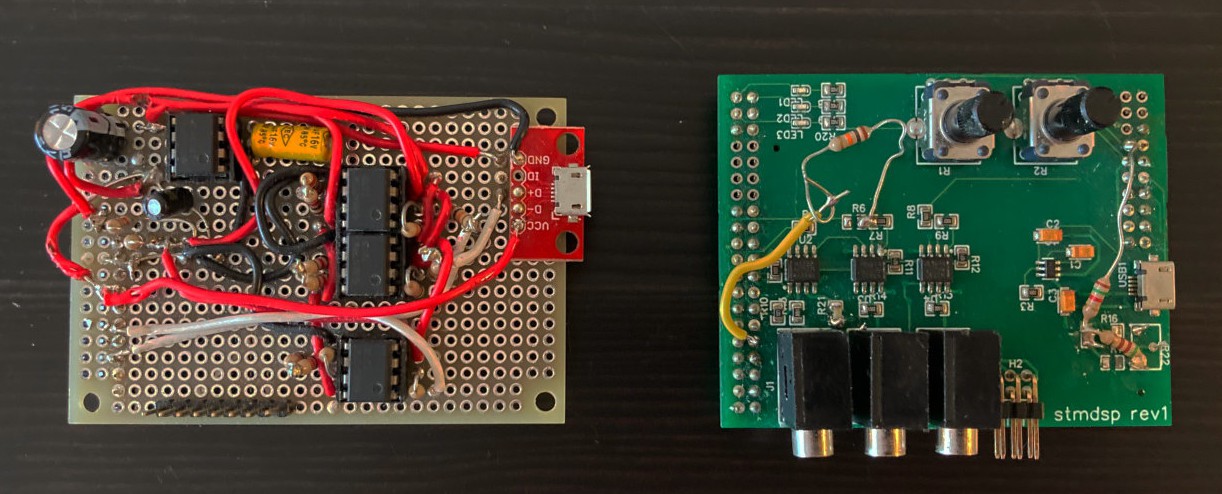
The DSP add-on board has gone through three iterations since the project's beginnings. It first started with a proto-board and DIP-socket ICs, then moved to a slightly-buggy PCB with surface-mount components:

The PCB implementation used a high-precision resistor divided to create a voltage reference; however, poor value/power choices led to the resistors burning out. Resistor adjustments also had to be made to the amplifiers to reduce some major signal noise. Additionally, the three status LEDs are facing south rather than up, a mistake in component selection.

The following revision (the current blue-PCB board) added a 3.3V reference, lower-noise operational amplifiers, and some signal filtering RC circuits. A couple of minor edits to this board has resulted in a reliable, high-quality add-on board.

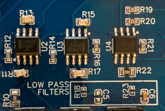
R11, R13, R15, and R17 have 220pF capacitors stacked on top to reduce high-frequency noise in the input and output signals. C5 was removed as the RC filter was not working as expected, instead distorted the signal. 

A final, fourth iteration is planned to build in these edits and produce a board that is ready for larger production and distributing to other users. Designing this iteration will also see a change in CAD software: the previous designs were done with EasyEDA, an online and proprietary solution linked to JLCPCB. This was chosen to simplify the production process, but is not ideal for more mature, open-source projects.

So, this iteration will be designed with KiCAD. This also means that the KiCAD project files can be added to the project's repositories, making it easier for others to work with hardware "source".