-
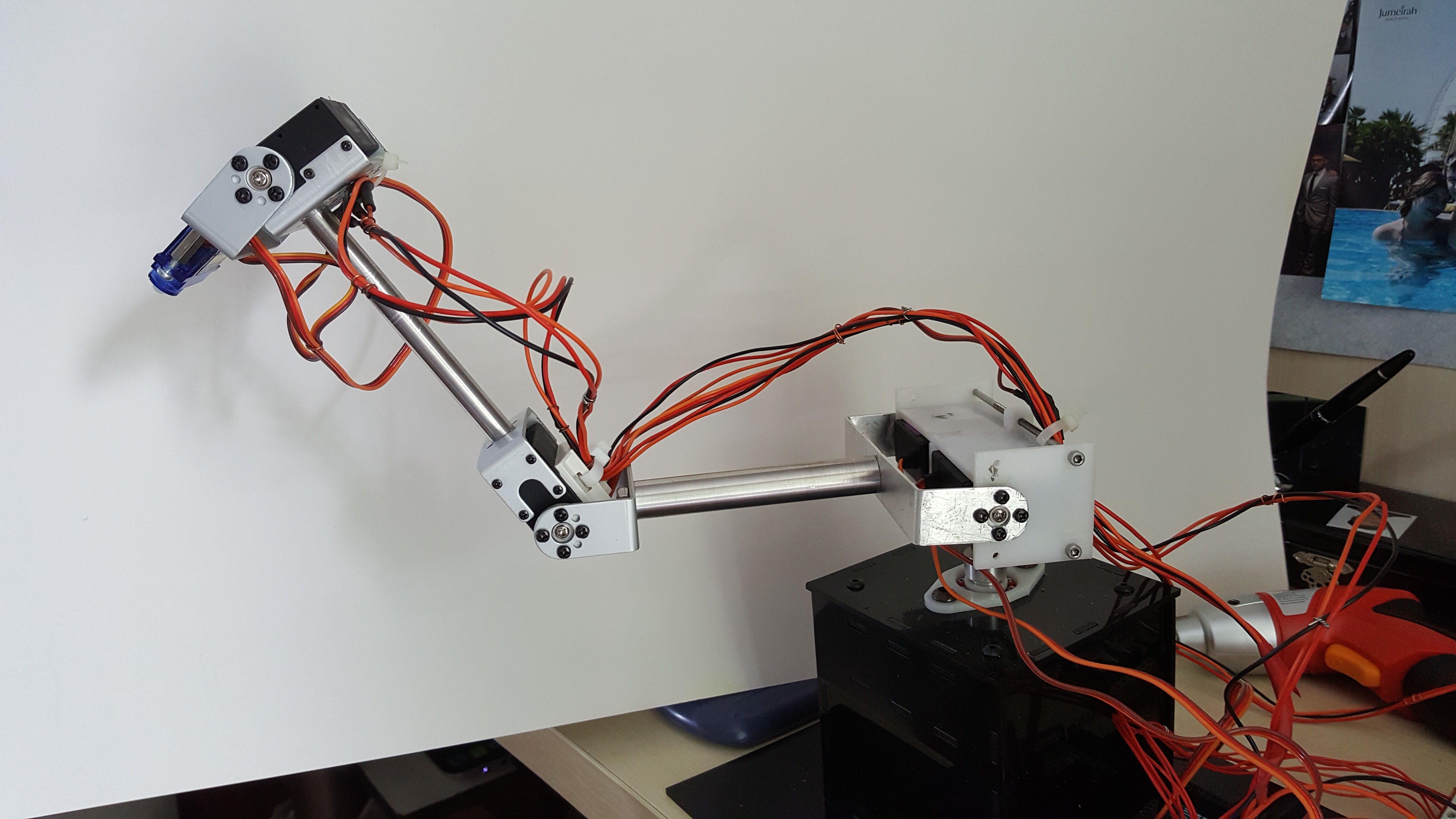
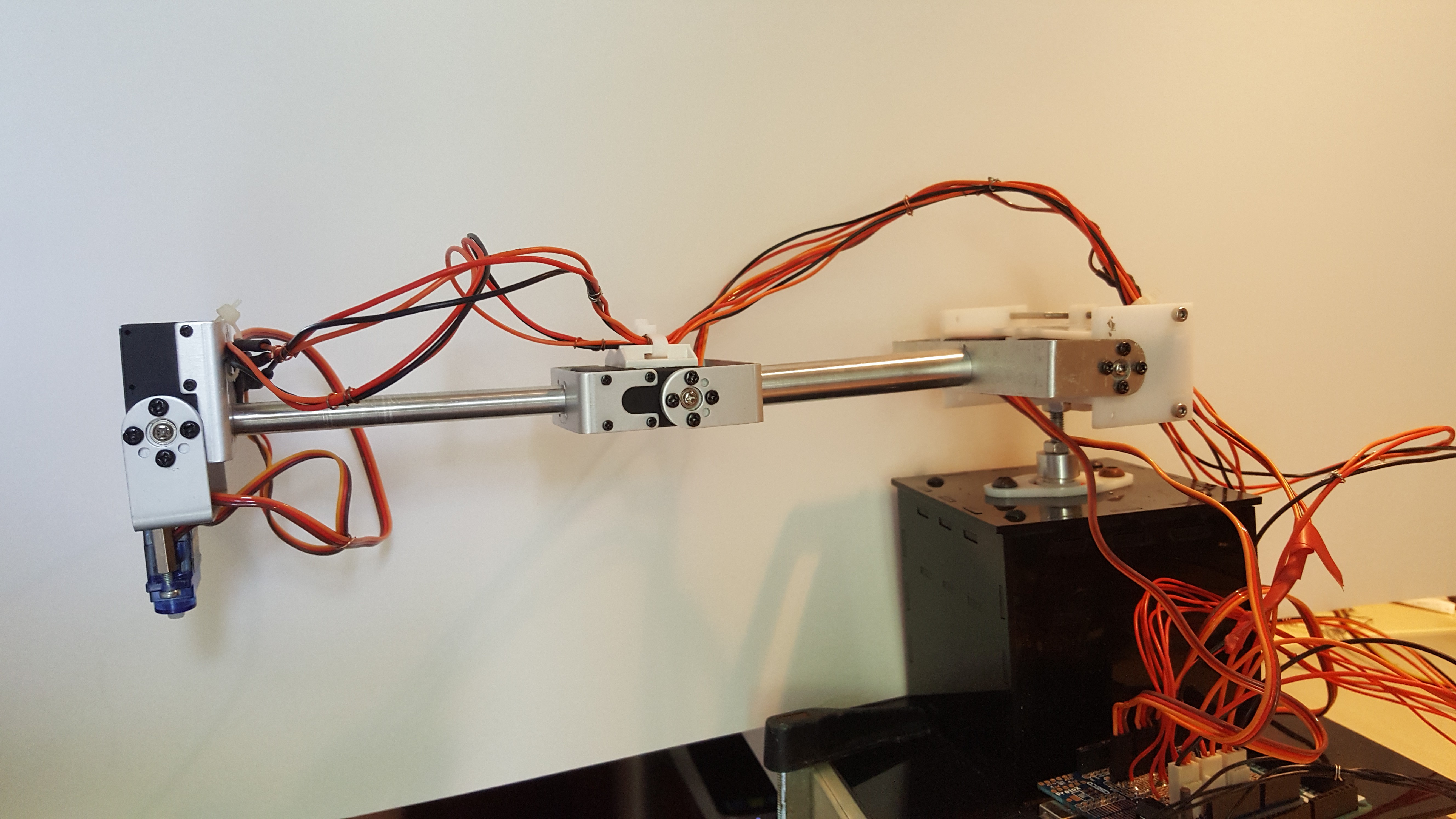
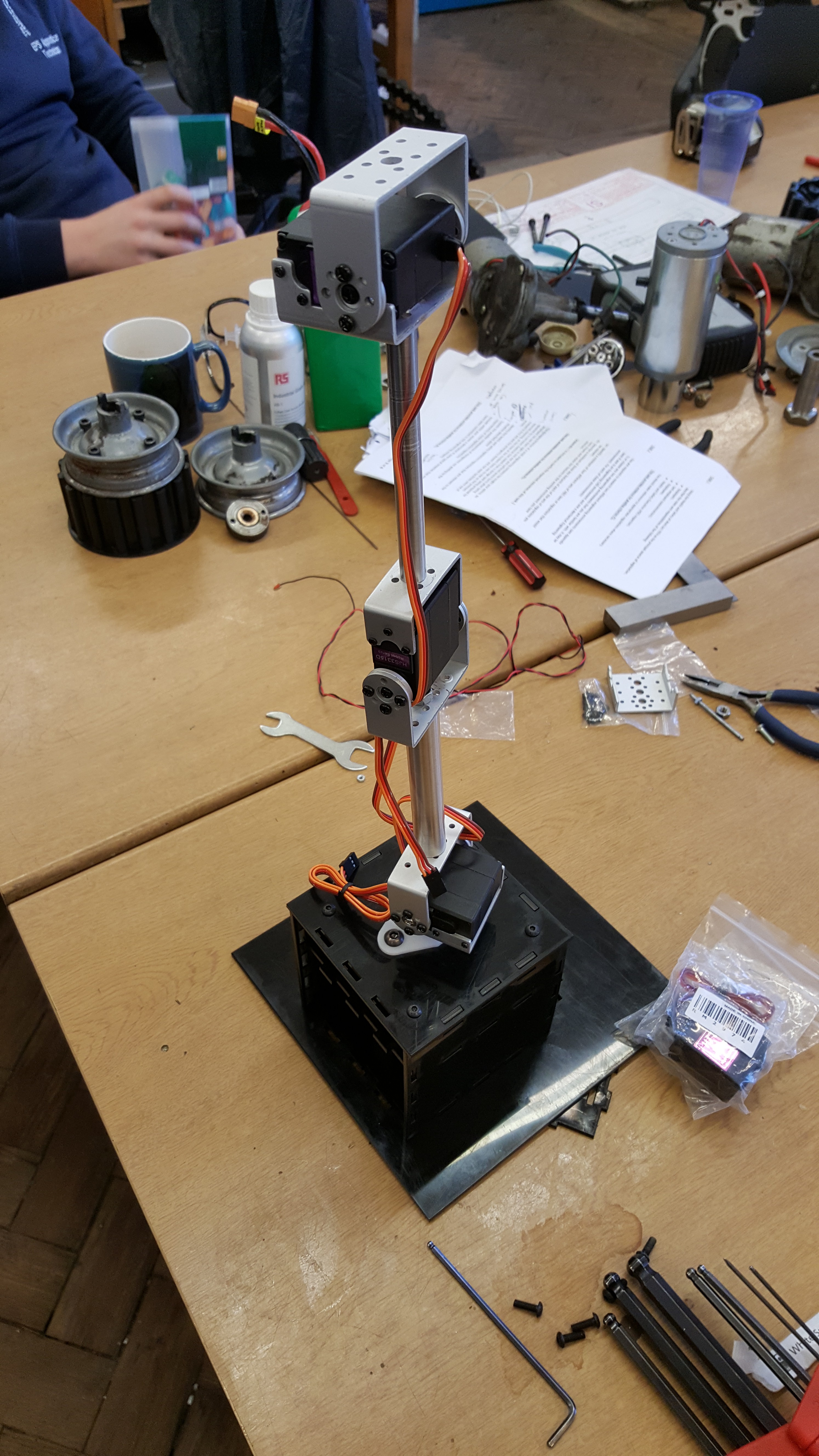
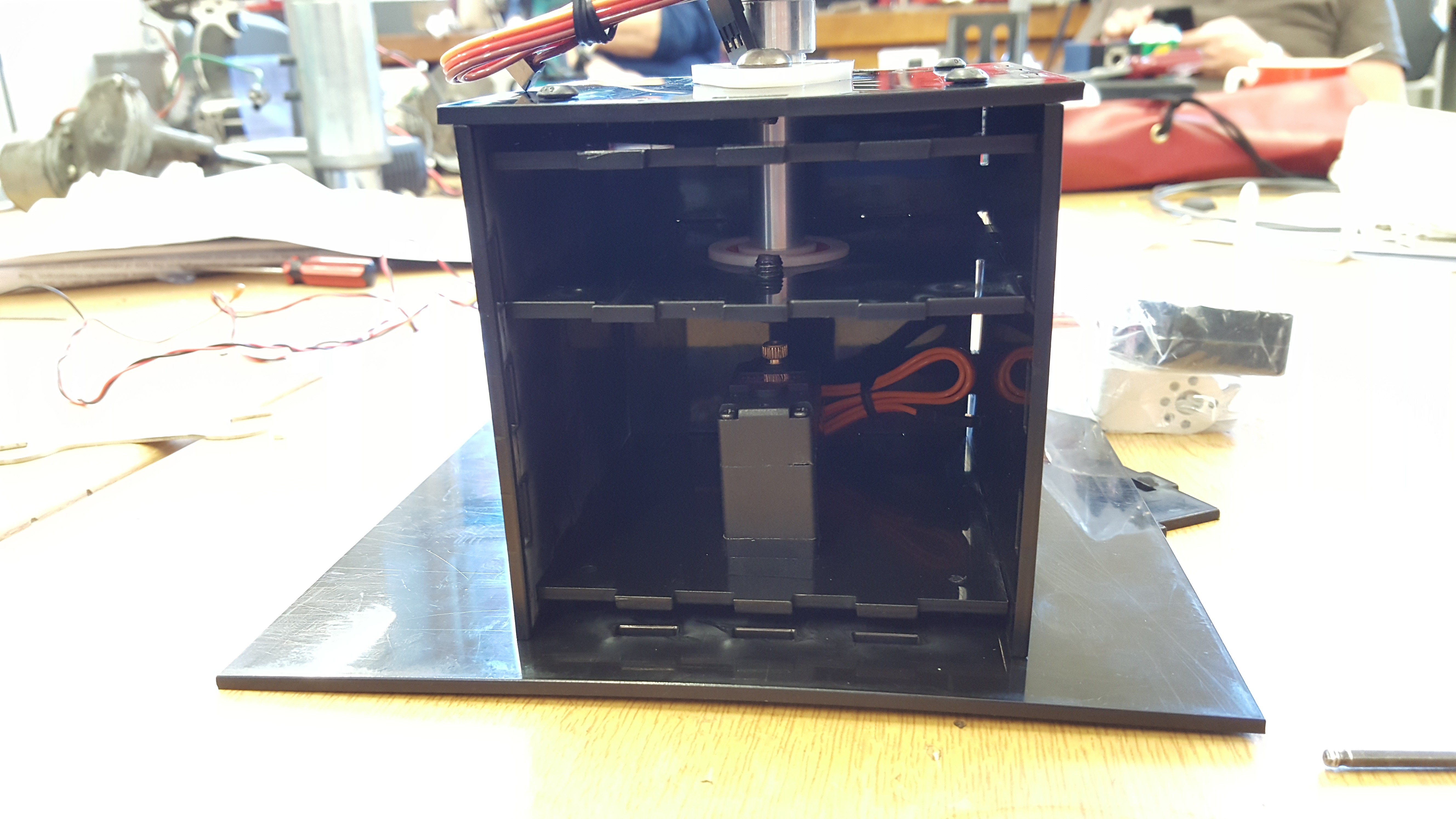
Assembly Completed
08/18/2017 at 11:10 • 0 comments -
MATLAB and Joystick
08/13/2017 at 22:25 • 0 commentsAs of know, the robot arm is fully functional and tested with the Serve Calibration code.
I have initially written the code on Arduino Web Editor but then installed an add-on to MATLAB and started using MATLAB to program my microcontroller. This is a huge advantage since all the computation is done on MATLAB (instead of the microcontroller) and MATLAB has a greater memory compared to the microcontroller.
Know we can control the robot arm (live time) using inverse kinematics. As the diagram in the appendix shows, the coordinate data will be inputted from a Joystick. The video below shows a quick demo.
-
Inverse Dynamics Controller
06/16/2017 at 13:58 • 0 commentsInverse dynamics is a nonlinear control technique that provides a better trajectory tracking by calculating the required joint actuator torques that need to be generated by the motors to achieve a given trajectory.
The matrix form of the dynamics of a robot leg is given by Equation 44 where the and terms are neglected.
 For a given and the non-linearity of the system can be vanished, making the system linear and hence the exact amount of torque that needs to be generated by the joint actuator to overcome the inertia of the actuator can be calculated. If the and match with the desired and then the projected trajectory will be tracked as expected [37].
Equation 45 shows the control law expression where is a new input to the system. The numeric value of is calculated by Equation 46 where is the desired trajectory, is the actual trajectory, and and are position and velocity gains, respectively [16].
Since the mass matrix, M, is invertible, equating Equation 45 to Equation 46 gives the expression in Equation 47 which shows that the new system is linear as it is given by Equation 48.
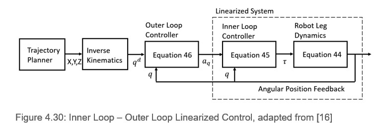
 Figure 4.30 demonstrates the inner loop and outer loop control architecture where the output of the system yields the joint space signal which enables a better trajectory tracking given that the feedback gains and are tuned as appropriate.
 -
Dynamic Model of Mechanical Drive Systems
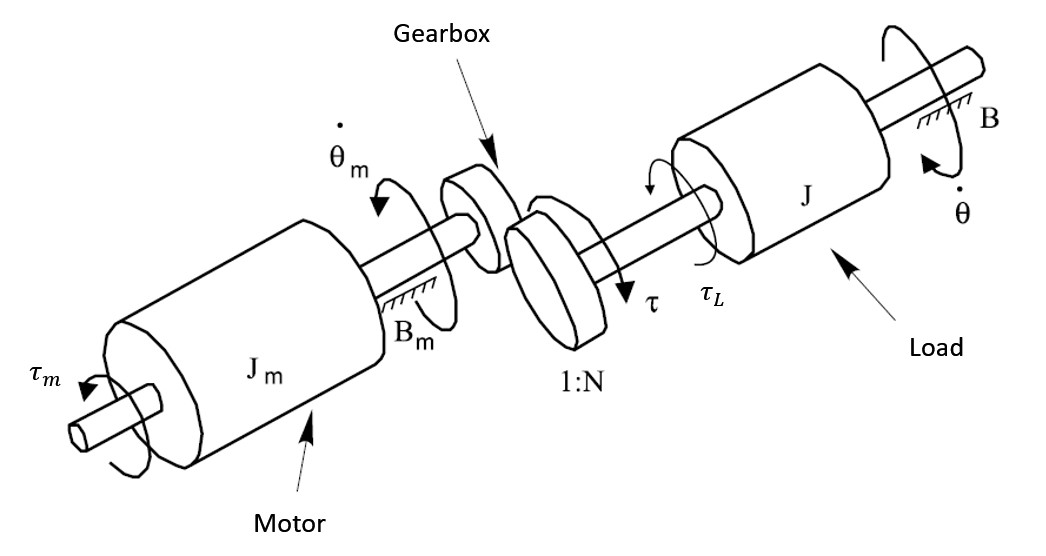
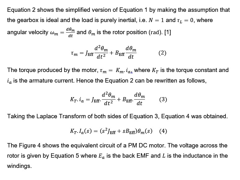
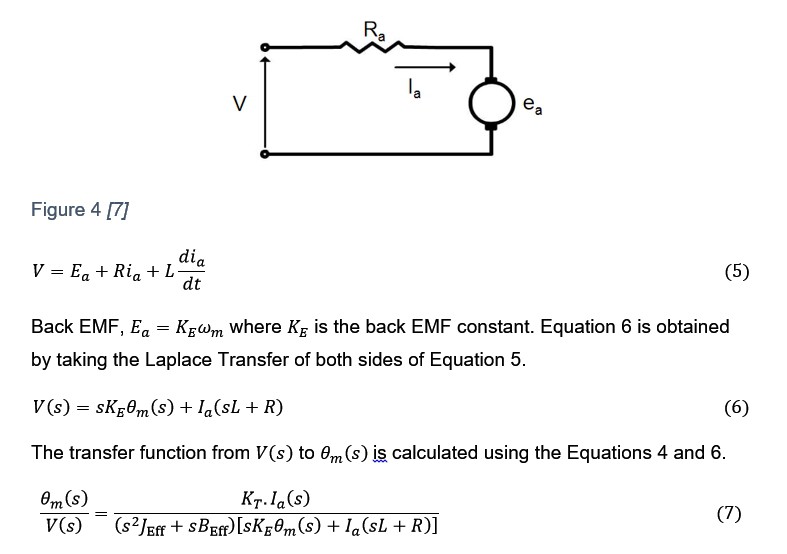
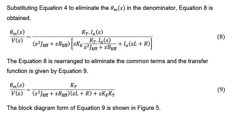
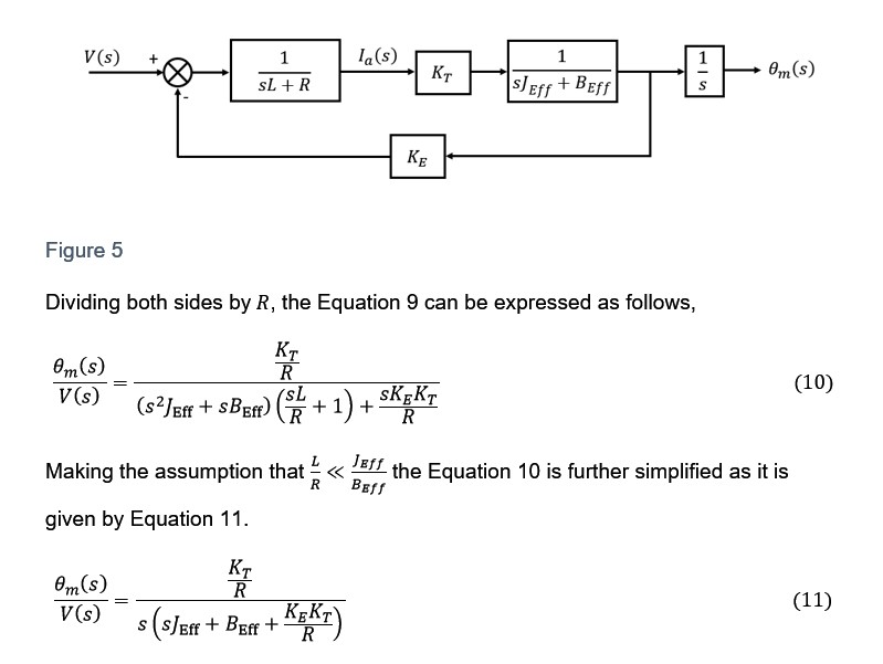
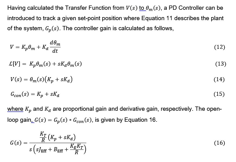
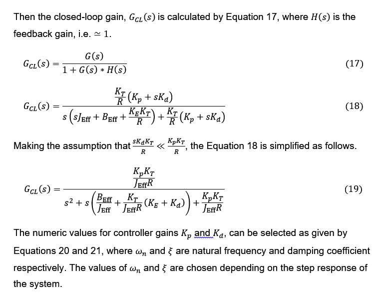
06/16/2017 at 13:45 • 0 commentsIn the MapleSim environment, the rotations of the revolute joints are controlled in joint space where are altered directly by applying signals to the joints. However, in real life, the rotation of the joint actuator is controlled by control signals, i.e. voltage or current. Therefore, the dynamic model of the motion system is crucial to deduce the relationship between the control signals and the rotation of the revolute joints. It is also used to obtain the relationship between control signal and joint actuator forces which serves the purpose of choosing the suitable actuators. The Figure 1 shows the mechanical model of a permanent magnet (PM) DC motor that is connected to an inertial load through a gearbox with a ratio of.
Figure 1
The fundamental mechanical relationship that defines the system in Figure 3 is given by Equation 1 which is also referred as torque balance equation
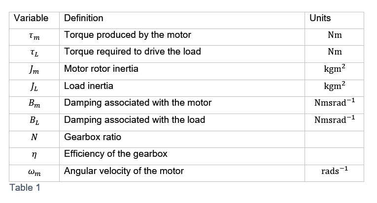
where the terms are given by Table 1.
Table 1
-
Test Trajectory
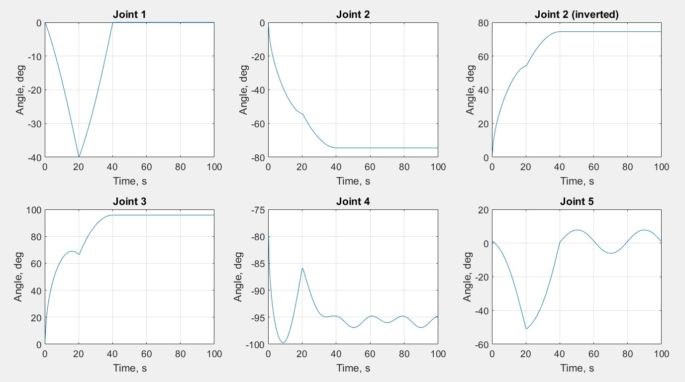
06/15/2017 at 09:50 • 0 commentsThe image below shows the trajectory that is used for testing the trajectory tracing of the robot manipulator. The Cartesian coordinates will be converted into joint rotations using the derived inverse kinematic equations, then these angles (CSV file) will be read using the Processing language.
The individual joint profiles are as follows,
-
Testing the Motors
05/27/2017 at 18:56 • 0 commentsIt can be seen in the video that the servo motors are configured and working. There is an undesirable vibration during the operation, that is because of using a potentiometer to control the angle of rotation. In reality, this will be done by a quintic trajectory planner which ensures a smooth motion when it is combined with a inverse dynamic controller. I will talk more about this in the following logs.
-
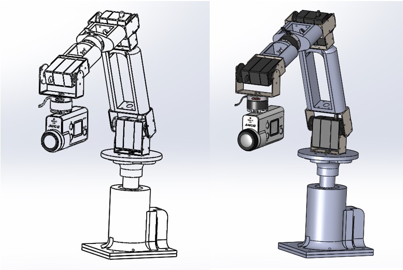
3D Design
05/13/2017 at 22:39 • 0 comments -
VR for Trajectory Generation
05/08/2017 at 20:16 • 0 commentsThe trajectory is generated on record and play basis. This is achieved by utilizing an open-source virtual reality software. An example is provided below.
-
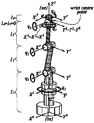
Kinematics
05/07/2017 at 14:53 • 0 comments -
Voltage Regulation Circuitry
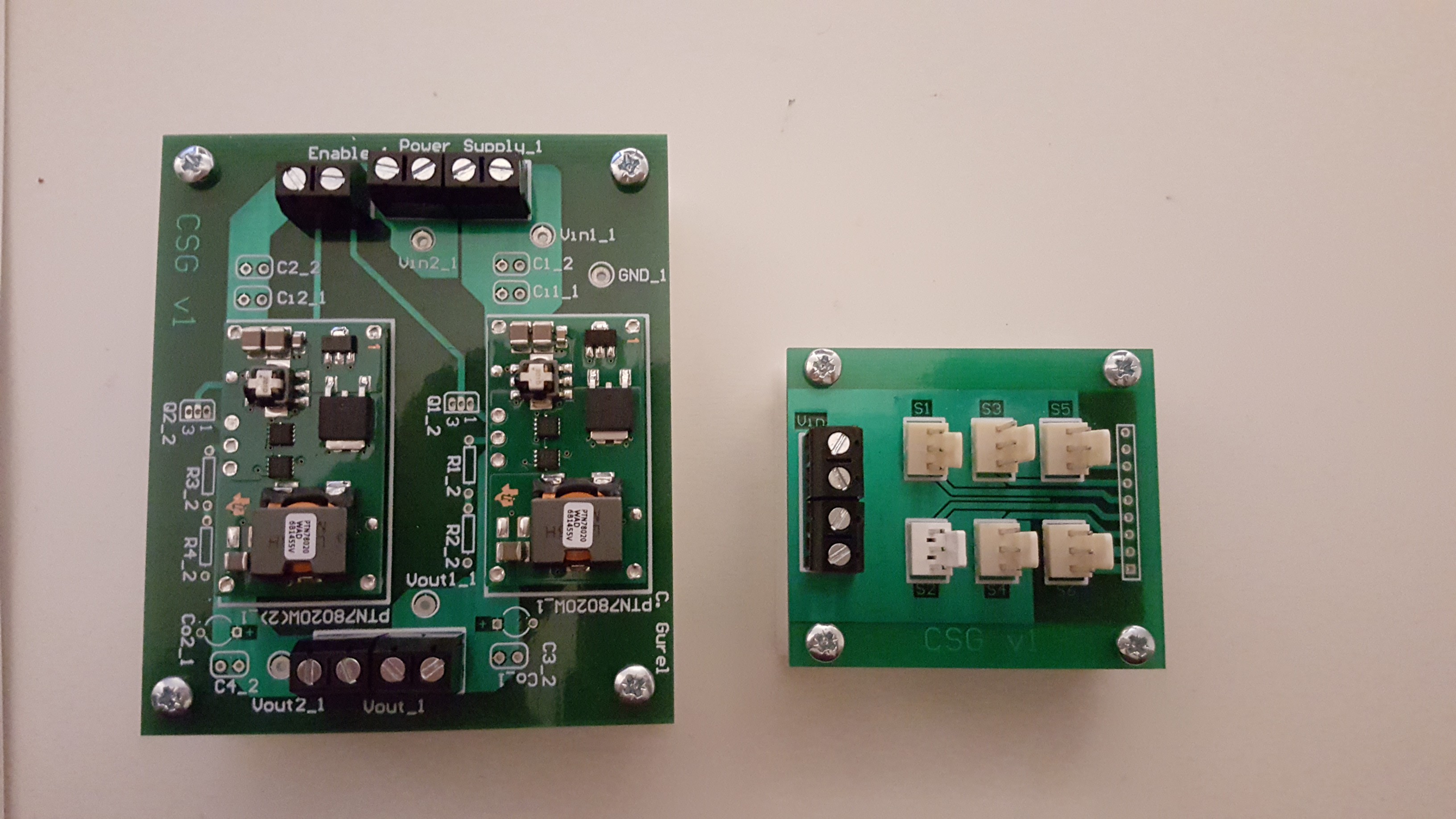
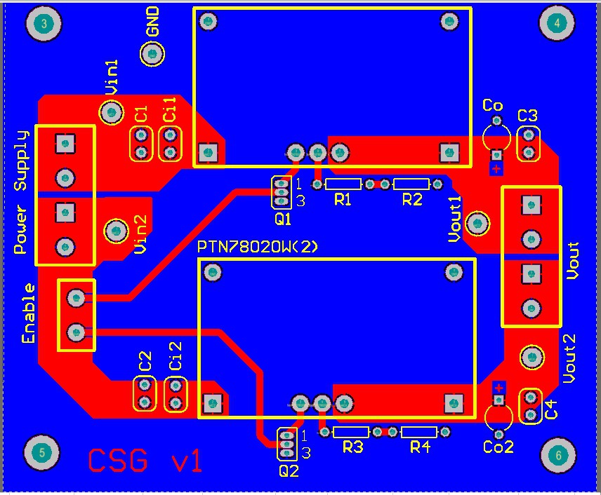
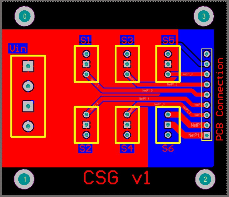
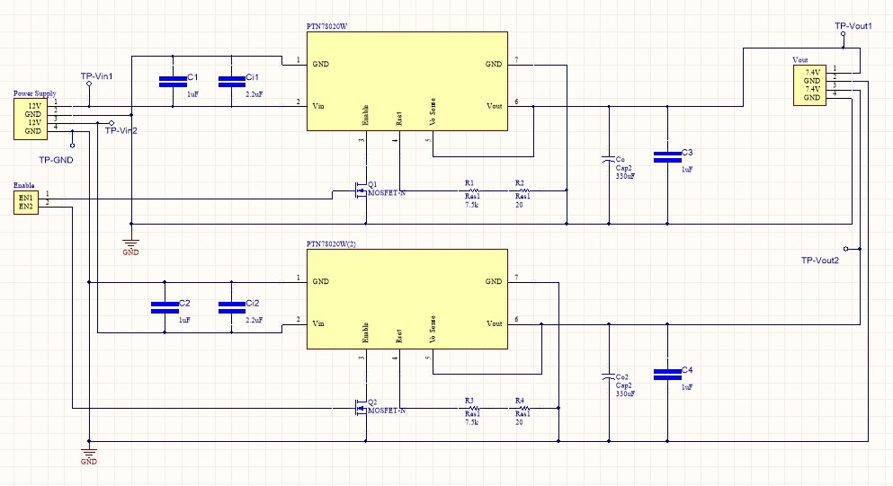
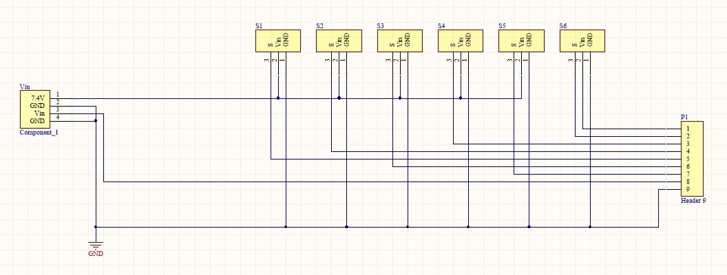
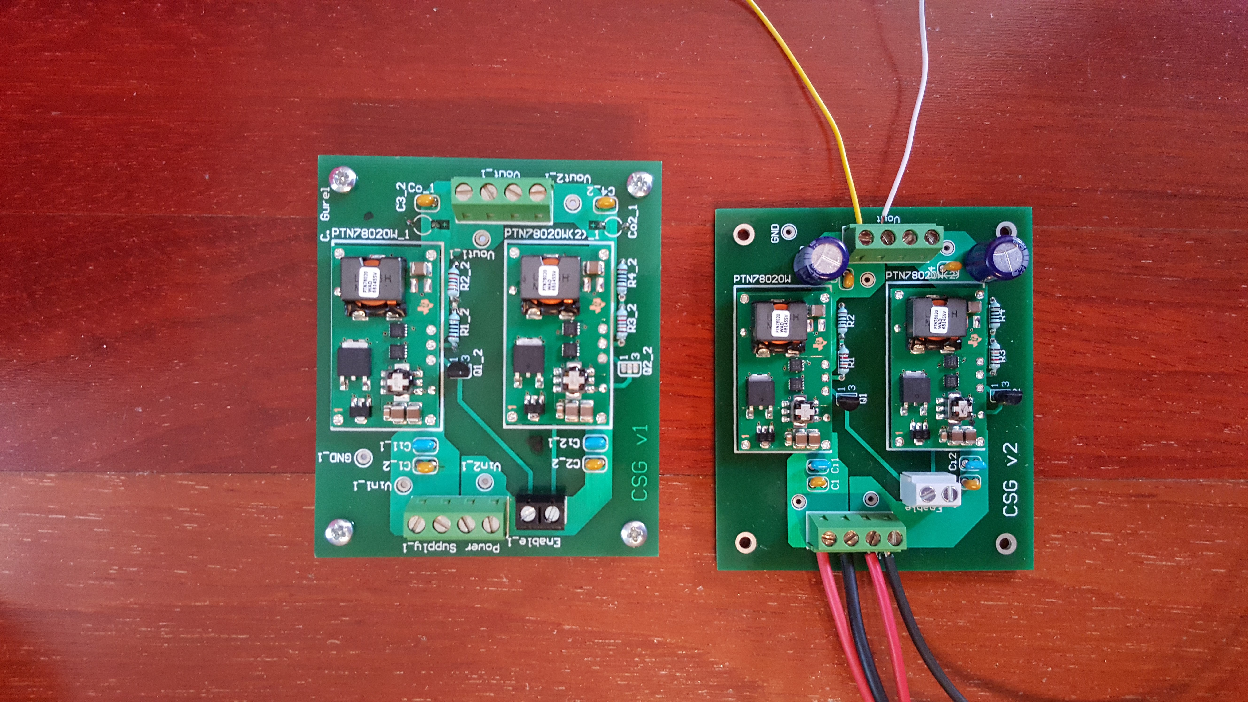
05/07/2017 at 14:31 • 0 commentsServo motors - as you can see from the datasheet provided in the Files - require 7.4V to operate at maximum torque of 16kgcm. However our experiments showed that motor windings got damaged due to high heat that had been generated. For this reason, I decided to supply 6V to each motor. The PCB on the left, consists of 2 step down converters. It supplies variable voltage that can be adjusted anywhere between 20V to 3V and maximum 6A. The PCB on the right is the connection to the motors.


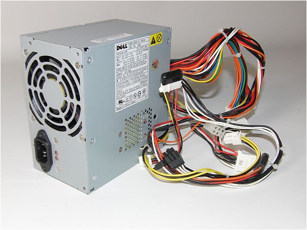
The circuits given above are supplied by a computer power supply which supplies 12V to each of the 4 step down converters. The datasheet of the converters are provided in the "files" section. The image below shows the computer power supply.
The following YouTube video is a tutorial that shows how it should be activated and connected to the rest of the circuitry.
Object Following Control of a Robotic Camera Arm
Virtual Reality, Kalman Filter, and Inverse Dynamics Control
