Tony Francis
-
Spectrometer Design: Tool Release- Optimal Slit Width Calculator
09/28/2025 at 19:37 • 0 commentsIf you followed the theoretical deep dive in our last log,Spectrometer Design Part 8: Calculating Optimal Slit Width, you know that determining the entrance slit width (w) is the final, crucial step in the optical design of the JASPER spectrometer. This single parameter defines the fundamental trade-off: light throughput vs. spectral resolution.
To make setting this parameter effortless for any design, we're excited to announce the release of the interactive tool:
The JASPER VIS/NIR Optimal Slit Width Calculator
What the Tool Does
This online calculator instantly computes the ideal slit width based on your design goals, ensuring your system's resolution is perfectly matched to your detector's pixel size.
The calculator:
- Explains the Math: It visually walks you through the four key steps (from the desired spectral resolution Δλ to the final equation) that were derived in the previous log.
- Solves the Equation: It uses the final derived formula, which elegantly links the physical slit width to your core design parameters:
Where:
- m = Diffraction Order
- Δλ = Target Spectral Resolution
- LC = Collimating Lens Focal Length
- d = Grating Groove Spacing
- β = Diffraction Angle
3. Provides an Interactive Interface: Just plug in your desired design values for spectral resolution, collimating lens focal length, grating grooves, and angle, and it instantly spits out the optimal slit width in micrometers (μm).
🖱️ Use the Calculator Now!
Whether you're building a JASPER or designing your own grating-based spectrometer, this tool will save you hours of manual calculation and help you lock in that perfect balance between light collection and spectrum clarity.
👉 Find the live tool here:
-
Spectrometer Design Part 8: Calculating Optimal Slit Width
09/26/2025 at 18:20 • 0 comments![]()
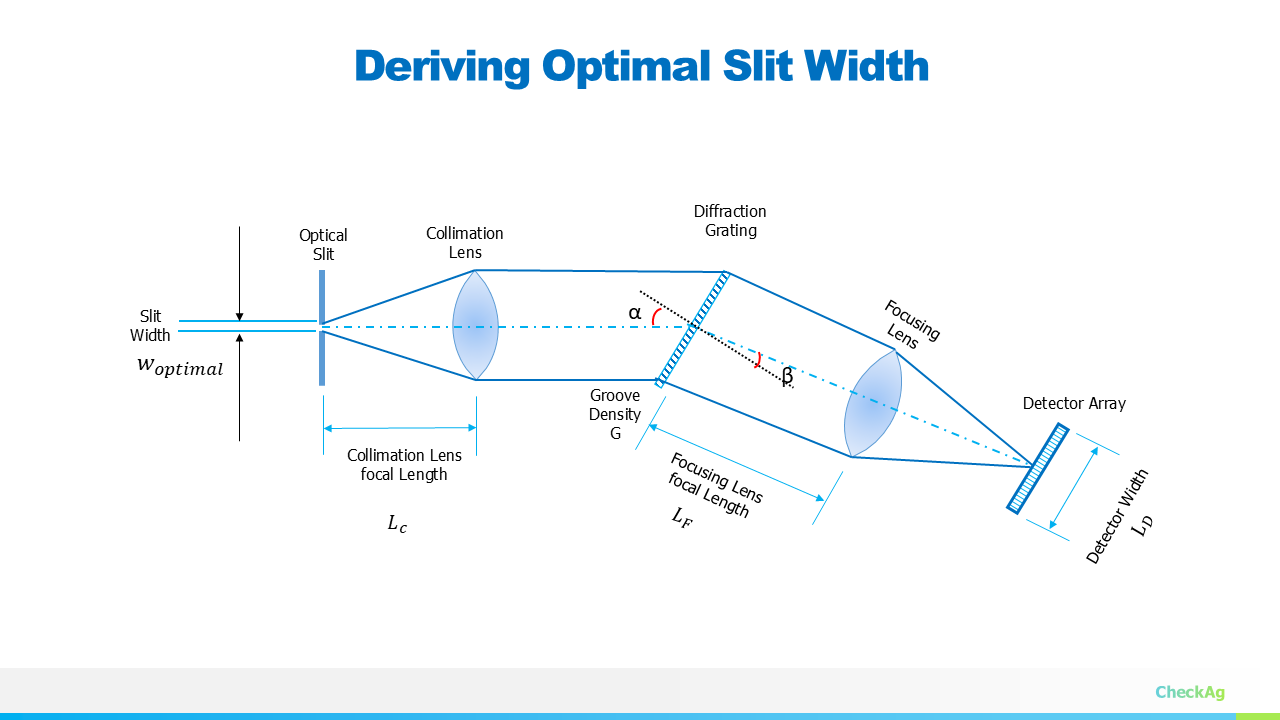
In our ongoing JASPER VIS-NIR spectrometer project, we have worked through the core components: fixing the geometry, selecting the grating, and deriving the focal lengths for the collimating (LC) and imaging (LF) lenses. The final piece of the optical puzzle is determining the optimal entrance slit width (w).
The slit width is critical because it directly controls the amount of light entering the system (the optical throughput) and also dictates the final spectral resolution. We need a slit that is wide enough to capture sufficient light but narrow enough not to degrade the resolution we designed the system for.
To find the optimal slit width, we must first recall the minimum required image size on our detector array.
Step 1: Minimum Resolvable Image Dimension (Δd)
The goal of any spectrometer is to distinctly separate two wavelengths that are very close to each other. This minimum difference in wavelength is our desired spectral resolution, Δλ.
For the spectrometer to register this change, the image of Δλ must be separated by at least two pixels on the sensor array. This means the minimum resolvable image dimension (Δd) must be equal to twice the pixel width.
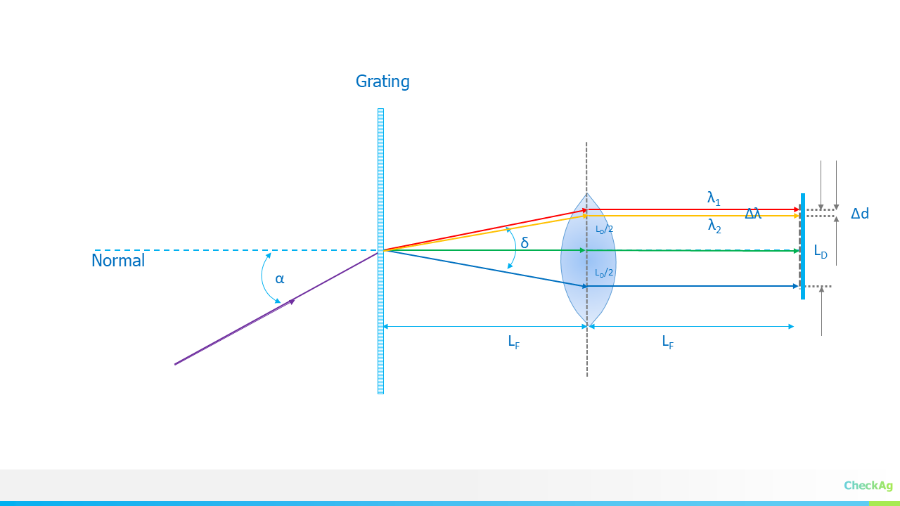
The relationship between the change in wavelength (Δλ) and the resulting physical separation on the detector (Δd) is governed by the linear dispersion of the system:
Note: The angular dispersion, dβ/dλ, which is the basis for this linear dispersion equation, was derived in detail in Part 6: Angular and Linear Dispersion https://hackaday.io/project/202421-jasper-vis-nir-spectrometer/log/243271-angular-and-linear-dispersion
where:
- m is the diffraction order (usually 1).
- LF is the focal length of the imaging (focusing) lens.
- d is the grating groove spacing.
- β is the angle of diffraction for the wavelength being resolved (often taken at λmin).
Solving for the smallest resolvable image dimension Δd at the desired spectral resolution Δλ:
For optimal performance, this dimension Δd should be set to match the physical requirement of the detector:
Step 2: Deriving the Optimal Slit Width (w)
In an infinity-corrected optical setup—where the collimating lens (LC) and the imaging lens (LF) are used—the slit width (w) is imaged onto the detector plane. The relationship between the object size (w) and the image size (Δd) is simply the ratio of the focal lengths of the two lenses:
We want the image of the slit to be exactly equal to our minimum resolvable image dimension (Δd) to ensure we utilize the maximum optical power without sacrificing resolution.
Now, we solve for the optimal slit width w:
Substituting the expression for Δd from Step 1 into this equation:
Notice that the focal length of the imaging lens,LF, cancels out, which significantly simplifies the final equation for the optimal slit width:
This final equation elegantly links the physical slit width to the core design parameters: the desired spectral resolution (Δλ), the grating characteristics (m and d), and the focal length of the collimating lens (LC). By setting the slit width according to this derivation, we achieve a system where the spectral resolution is perfectly matched to the detector's pixel size, thereby optimizing both light throughput and resolution.
In the next part, we will use all these derived equations to plug in our target values and finalize the physical dimensions of the JASPER spectrometer.
-
Part 7: Deriving the Focal Length of a Collimation Lens
09/24/2025 at 18:48 • 0 commentsIn our last post, we discussed how to select the right detector length and focusing lens. Now, we're going to dive into the optics of the grating itself, specifically how it affects magnification in your system.
The Anamorphic Nature of a Grating Spectrometer
A grating spectrometer is an anamorphic optical system, which means it magnifies in different ways along different axes. To briefly review this property, assume the entrance aperture of the spectrograph is a slit of width W and length L, aligned so that its projected image lies perpendicular to the direction of dispersion. The projected length l at the detector is then:
where FF; and FC; are the focal lengths of the imaging lens and collimating lens, respectively.
However, there's another crucial magnification at play—the magnification in the direction of the dispersion. This is a direct result of how light interacts with the grating.
Deriving the Magnification from the Grating
![]()
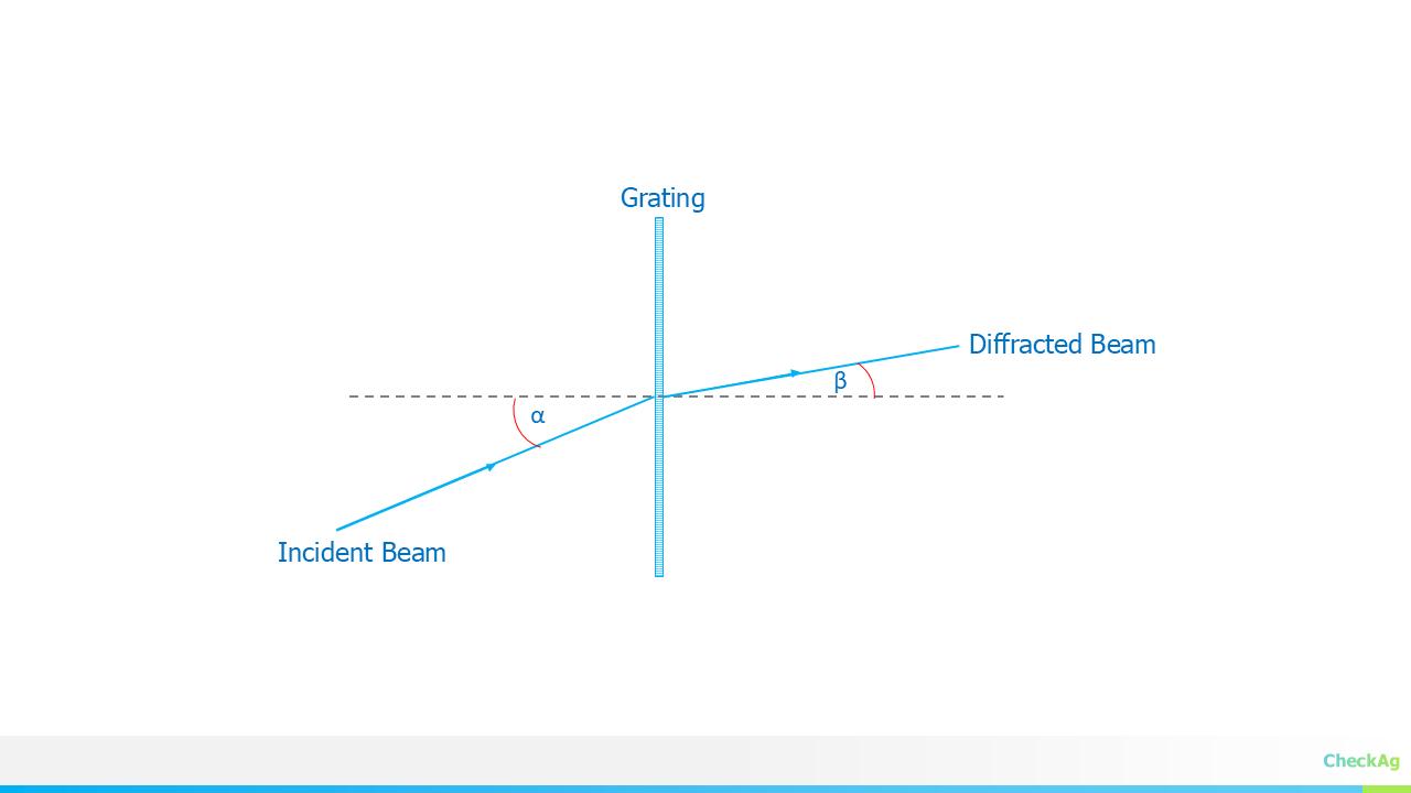
To understand, let's consider the grating equation, which describes the relationship between the angles of the incident and diffracted light.
where:
- m is the diffraction order
- λ is the wavelength of light
- d is the groove spacing of the grating
- α is the angle of the incident ray with respect to the grating normal
- β is the angle of the diffracted ray with respect to the grating normal
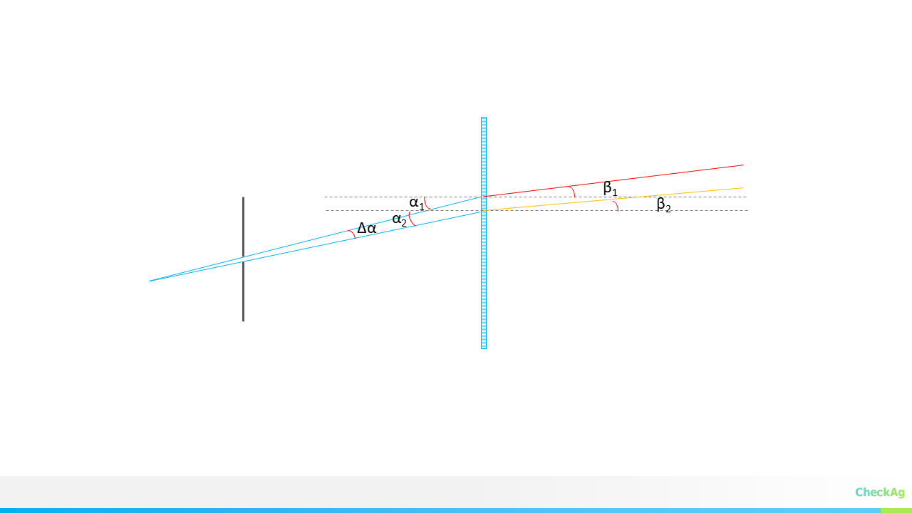
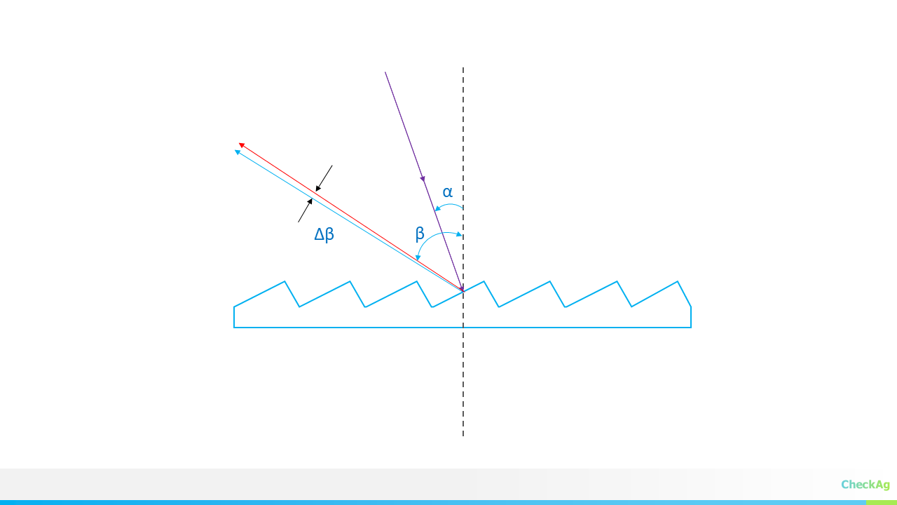
Now, let’s consider two rays originating from opposite edges of the entrance slit. These two rays arrive at the grating with incident angles that differ by a small amount, Δα. After passing through the grating, the diffracted rays will leave with an angle difference of Δβ, where Δβ ≠ Δα.
![]()
The magnification of the grating, r, is defined as the ratio of these two angular changes:
To find the relationship between Δβ and Δα, we can differentiate the grating equation with respect to α and β, while assuming the wavelength (λ) is constant.
Let's start with the grating equation:
Since m, λ, and d are constants for a single wavelength, their product is also a constant. Therefore, the derivative of the left side of the equation is zero. We can differentiate the right side with respect to α and β:
Using the chain rule, this becomes:
Rearranging the terms to solve for the ratio of dβ to dα, we get:
The magnification, r, is the ratio of the change in the diffracted angle to the change in the incident angle. In the limit of very small changes (Δα and Δβ), we can replace dβ/dα with Δβ/Δα. Since magnification is typically concerned with the magnitude of the angular change, we take the absolute value:
This term, cosα / sinβ, is the anamorphic magnification factor of the grating itself
Putting It All Together: The Total Magnification
The overall magnification (M) of the spectrometer is the product of the magnification from the lenses and the magnification from the grating. Therefore, the total magnification is:
From this, you can solve for the focal length of the collimating lens Fc :
In practical spectrometer design, a magnification (M) close to 1 is often targeted to maintain a one-to-one relationship between the slit and the detector image.
In the next post, we'll discuss the final component of our optical system: the entrance slit, and how its width impacts the spectral resolution of your spectrometer.
-
Part 6: An Interactive Tool for Selecting Spectrometer's Focusing Lens and Detector
09/18/2025 at 18:47 • 0 commentsIn the last blog post, we delved into the theoretical foundations of spectrometer design, particularly the relationship between spectral resolution and detector pixel size.
Building on that, we have designed a new tool to help you tackle a critical design challenge: selecting the perfect combination of a focusing lens and a detector.
The Problem: A Catch-22 in Spectrometer Design
When you're designing a spectrometer from scratch, you quickly realize you're faced with a classic "chicken-and-egg" problem. The required length of your detector is directly dependent on the focal length of your focusing lens, and vice versa. Since both are unknown at the beginning, it's difficult to know where to start. Customizing a lens is prohibitively expensive, so you have to work with standard, off-the-shelf components.
To solve this, we've developed a practical, iterative approach. Our tool lets you choose a standard focal length from a list of commercially available lenses. It then calculates the exact detector length you would need to capture your full wavelength range. From there, you can choose the closest-matching detector from a catalog.
Introducing the Interactive Design Calculator
Our new web-based calculator takes the guesswork out of this process. It's a single-page application that allows you to experiment with your design parameters in real-time.
Try it out here:
https://checkag.github.io/detector_and_focusing_lens/
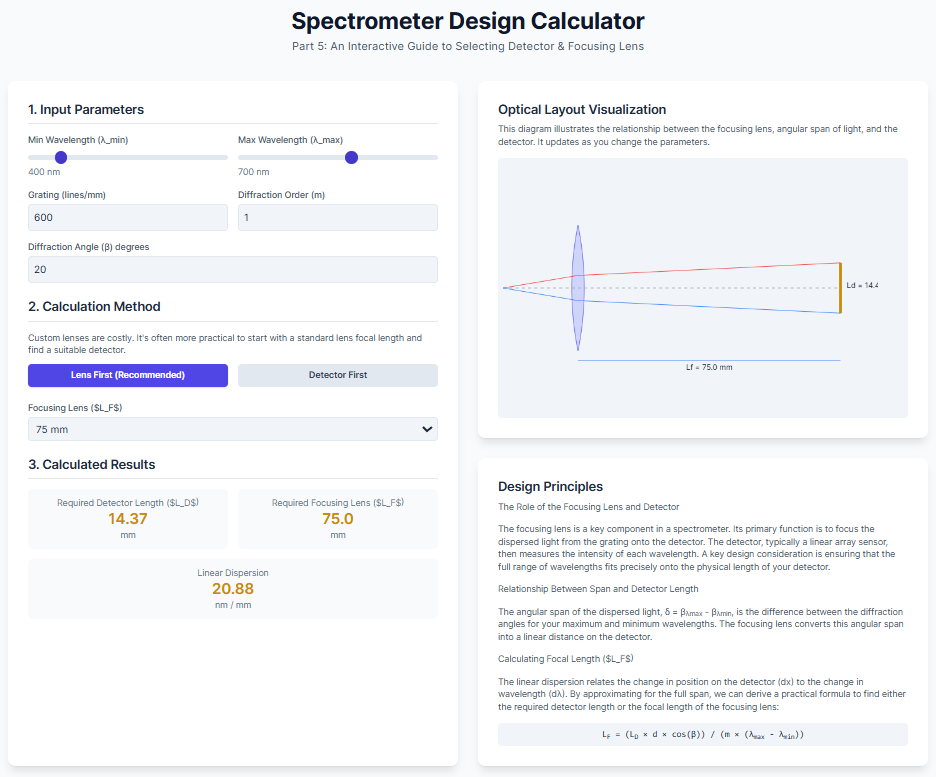
A snapshot of the design tool:
![]()
How it works:
- Input Parameters: Enter your desired wavelength range (λmin to λmax), grating specifications (lines/mm), and diffraction order.
- Practical Approach: Select a standard focal length for your focusing lens from the dropdown menu.
- Real-time Visualization: Watch as the tool instantly calculates the required detector length. The interactive diagram on the right updates to visually demonstrate the effect of your choices on the spectrometer's geometry.
This interactive tool is a significant step forward in our project, turning complex equations into a straightforward, visual experience. We believe this will be incredibly useful for anyone building their own spectrometer.
-
Part 5: A Guide to Selecting Detector Length and Focusing Lens for grating Spectrometer
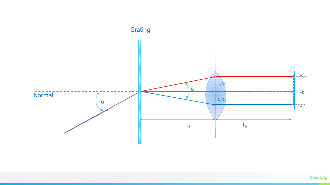
09/16/2025 at 19:05 • 0 commentsIn our last blog post, which you can find here, we discussed the concept of spectral resolution and its direct relationship to the pixel size of the detector. In this post, we will discuss how to select detector length and the focal length of the imaging lens, which are crucial for the instrument's performance.
![]()
1. The Role of the Focusing Lens and Detector
The focusing lens (also known as the imaging lens) is a key component in a spectrometer. Its primary function is to focus the dispersed light from the grating onto the detector. The detector, typically a linear array sensor, then measures the intensity of each wavelength.
A key design consideration is ensuring that the full range of wavelengths you want to measure (λmin to λmax) fits precisely onto the physical length of your detector.
2. The Relationship Between Wavelength Span and Detector Length
The angular span of the dispersed light, δ=βλmax−βλmin, is the difference between the diffraction angles for your maximum and minimum wavelengths. The focusing lens converts this angular span into a linear distance on the detector.
The relationship between the detector length (LD), the focusing lens's focal length (LF), and the angular span (δ) is given by the following equation:
This equation highlights the trade-off: for a fixed angular span, a longer focal length (L_F) will result in a larger image on the detector, requiring a longer detector.
3. Calculating the Focusing Lens Focal Length (L_F)
Often, the detector length (L_D) is a known value—you have a specific sensor you are designing around. To find the required focal length of the focusing lens, we can rearrange the equation above.
The angular dispersion describes how much the diffraction angle changes with a change in wavelength. It's defined as:
- m: The diffraction order
- d: The groove spacing of the grating
- β: The diffraction angle
The linear dispersion, which relates the change in position on the detector (dx) to the change in wavelength (dλ), is given by:
We can approximate the linear dispersion for the full wavelength span. The change in position, dx, corresponds to the detector length, LD, and the change in wavelength, dλ, corresponds to the wavelength span, λmax−λmin.
Rearranging this equation to solve for the focal length of the focusing lens (LF), we arrive at the formula :
This equation provides a direct and practical way to calculate the required focal length of the focusing lens based on your detector length, grating parameters, and the desired wavelength range.
Practical Approach
Since both the detector length and the focusing lens focal length are unknowns in the spectrometer design, a common and practical approach is to fix one of them to find the other.
In practice, it can be challenging to find a detector with the exact length calculated above. Also, customizing a lens is costly, and stock lenses have standard focal lengths like 30mm, 50mm, 75mm, 100mm etc. Therefore, a more practical procedure is to calculate the detector length for the available focal lengths and then select the most optimal detector-focal length combination.
- Select a Trial Focal Length: Choose a commercially available focal length for your imaging lens. Common options are 30mm, 50mm, 100mm, 150mm, 200mm, etc. A longer focal length will result in a longer detector length and higher spectral resolution.
- Calculate the Required Detector Length: Using the focal length you've selected, plug the values for the other known parameters (m, d, β, and the wavelength span) into the equation above to calculate the required detector length,LD.
- Choose a Close Detector: Compare your calculated LD to the available sizes of commercial detectors. Select a detector that is the closest match to your calculated value.
By following this method, you can start with a standard component (the lens) and then find a detector that is a good fit for your system's required wavelength span and spectral resolution.
-
Spectrometer Design Part 4: Spectrometer design with sensor array
09/15/2025 at 19:49 • 0 commentsIn our previous blogs, we tackled the initial steps of designing a spectrometer: fixing the geometry ϕ=α+β and then calculating the angles of incidence (α) and diffraction (β). We even created a simulator that showed how a varying α could achieve a desired spectral range. Details at
https://hackaday.io/project/202421-jasper-vis-nir-spectrometer/log/243174-spectrometer-design-part-3-deriving-alpha-and-beta-angles
https://hackaday.io/project/202421-jasper-vis-nir-spectrometer/log/243185-simulating-diffraction-gratingWhile a rotating grating-based monochromator offers supreme flexibility—allowing for variable spectral resolution or even the use of multiple gratings on a turret—it is not the optimal choice when spectral acquisition speed is paramount.
For high-speed spectroscopy, the ideal solution is a spectrometer with a stationary grating and a sensor array detector. This design has no moving parts and relies on a constant angle of incidence (α). The entire spectral range is imaged simultaneously onto the array, where each pixel corresponds to a specific wavelength.
Let's explore the key equations that govern this design.
The Grating Equation for a Fixed-Grating System
The fundamental grating equation is:
Here, m is the diffraction order, λ is the wavelength, and d is the grating groove spacing. For a fixed-grating system, α is constant. We can derive the equation for the diffraction angle β as a function of wavelength:
The total spectral span captured by the detector is the difference in diffraction angles between the maximum and minimum wavelengths of interest, λmax and λmin.
From Angular Dispersion to Physical Dimensions
![]()
The spectral span δ is an angular measurement. We must convert this into a physical length that can be imaged onto the detector. This is where the imaging lens and its focal length (LF)come into play. The total length of the detector (dD) required to capture the entire spectral span is given by:
This equation highlights the trade-off between the detector's physical size and the focal length of the imaging lens. The span is limited by these two parameters.
To determine the smallest change in wavelength (Δλ) that the spectrometer can resolve, we need to consider the angular dispersion, which describes how the diffraction angle changes with a change in wavelength.
For a very small change, we can approximate this relationship as:
This angular change, Δβ, must be large enough to be detected by the sensor. The smallest resolvable image dimension (Δd) on the detector corresponds to the spectral resolution. This allows us to select a detector with an appropriate pixel size. The linear dispersion is given by:
The physical distance between two adjacent resolvable wavelengths is Δd. To distinctly record two close spectral lines, they must be mapped onto two adjacent pixels.
In practice, a design workflow is typically reversed. We start with a fixed pixel size and sensor length from available detectors and work backward to calculate the achievable spectral resolution. If the result doesn't meet the design goals, we can iterate on other parameters like the angle of incidence (α) or the grating's groove density.
This shows that even with a fixed grating, there are many parameters to tune for an optimal design. In the next blog, we can create a simulator to compute the pixel size required for a given spectral resolution and span, bringing these equations to life
-
Angular and Linear Dispersion
09/10/2025 at 19:32 • 0 commentsAt the core of the JASPER VIS-NIR spectrometer is a diffraction grating, a component with thousands of microscopic grooves. When light hits this grating, it is diffracted, with each wavelength bent at a different angle. This is governed by the Grating Equation:
Here, λ is the wavelength of light, d is the spacing between the grating grooves, m is the diffraction order, α is the angle of incidence, and β is the diffraction angle. For a given setup, d, m, and α are constant.
![]()
The measure of how well the grating separates different wavelengths is called angular dispersion, defined as the change in diffraction angle (β) for a small change in wavelength (λ). We can find this by differentiating the grating equation with respect to λ:
This simplifies to:
Rearranging for the angular dispersion, we get the corrected equation:
A higher value for dβ/dλ means that two very close wavelengths will exit the grating at noticeably different angles, which is exactly what we want for a high-performance spectrometer
From Angle to Position: The Role of Linear Dispersion
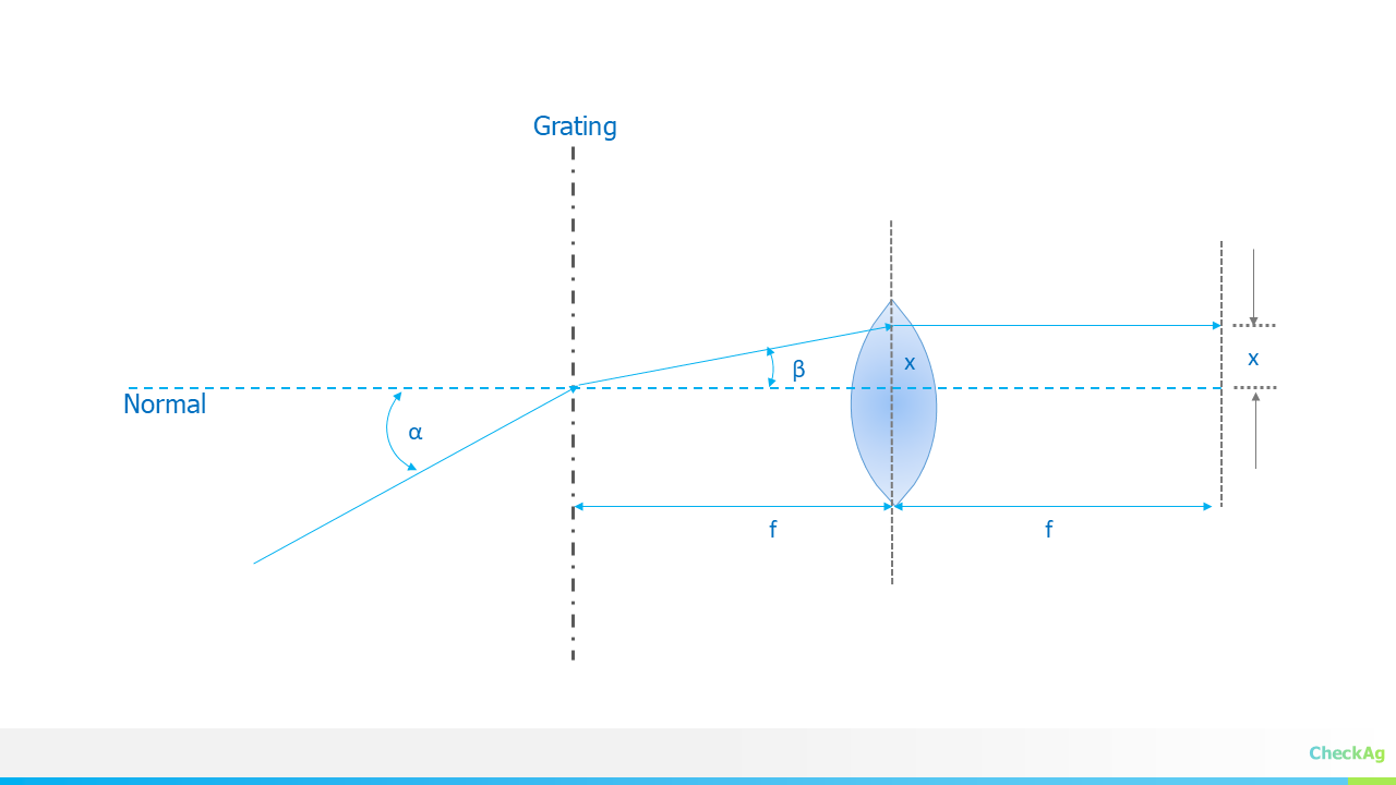
After the light is separated by angle, it passes through a lens that focuses the diffracted rays onto a detector plane, such as a CCD or CMOS sensor.
![]()
This lens transforms the angle (β) into a specific position (x) on the detector. The relationship is given by:
where f is the focal length of the focusing lens. This equation is accurate for a flat detector plane normal to the central ray.
To understand how a change in wavelength relates to a change in position on the detector, we need to combine the two concepts. The key metric for a spectrometer is its linear dispersion, dx/dλ, which tells us how many nanometers of wavelength are spread across one millimeter of the detector
Using the chain rule, dλ/dx=(dλ/dβ)⋅(dβ/dx). We can derive the expression for linear dispersion:
This equation is a cornerstone of spectrometer design. A lower value of dλ/ corresponds to a higher resolution, meaning the spectrometer can distinguish between very closely spaced wavelengths. This is achieved by using a grating with a small groove spacing (d), operating at a higher diffraction order (m), or using a lens with a longer focal length (f)
-
Simulating Diffraction Grating
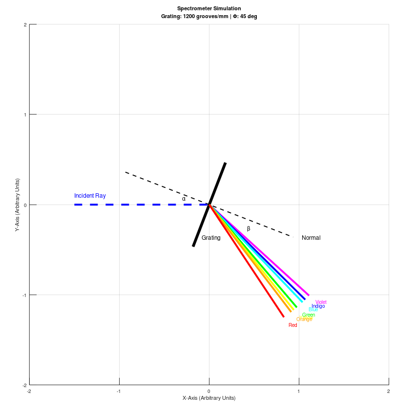
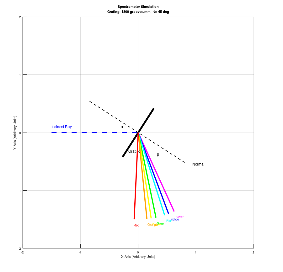
09/06/2025 at 11:25 • 0 commentsIn our previous blog post, we detailed the fundamental geometry of our spectrometer, where the angles of incidence (α) and diffraction (β) are derived from a single geometric parameter, Φ. To bring this theory to life, we've created an Octave script that visually simulates how a diffraction grating splits light into its constituent colors based on this very principle. This script serves as a powerful educational tool to understand the physics at play.
The core of this simulation lies in the equations we derived:
Our script uses these formulas to calculate the diffracted angles for a range of wavelengths across the visible spectrum (VIBGYOR). By setting a fixed value for and the grating's groove density, the code plots a representation of the grating, the incident light ray, and the distinct diffracted rays for each color. This approach, where a single parameter defines the geometry, is often employed in a monochromator setup where the grating rotates to select a specific wavelength.
It's important to note that while this simulation is excellent for educational purposes, our final spectrometer design employs a different strategy. Our practical design will feature a fixed angle of incidence (α), and the diffracted light will be captured by a stationary photodiode array. The choice of the detector's position is a critical design step to capture the wavelengths of interest. Therefore, while our simulator highlights the beautiful physics of a rotating grating, it is not a direct model of our final instrument.
As an example of the output of the published code, we share three example configurations demonstrating the effect of grating groove density on diffraction angle and the diffraction angle placement.
Example Configurations
Phi = 45 and grating groove density = 600 l/mm
![]()
Phi = 45 and grating groove density = 1200 l/mm
![]()
Phi = 45 and grating groove density = 1800 l/mm
![]()
We encourage you to experiment with the code by changing the value of Φ or the Grating_Density. This will allow you to see firsthand how these parameters directly influence the angles of incidence and diffraction, and ultimately, the spectral output.
% This Octave script simulates a spectrometer, plotting the incident ray and % the diffracted rays for the visible spectrum (VIBGYOR). The simulation % is based on the grating equation and a non-zero angle of incidence. % --- Input Parameters (Editable) --- % Angle Phi in degrees. This angle defines the overall geometry of the % spectrometer, influencing both the angle of incidence and diffraction. % Based on the derivation at hackaday.io/project/202421-jasper-vis-nir-spectrometer/log/243174-spectrometer-design-part-3-deriving-alpha-and-beta-angles Phi_deg = 45; % User-defined Phi angle in degrees. Phi_rad = deg2rad(Phi_deg); % Convert to radians for calculations. % Diffraction grating parameters. m = 1; % Diffraction order (set to 1 as per request). % Grating groove density (lines per mm) to grating period 'd' (in meters) % Uncomment the desired value below to change the grating. Grating_Density = 1800; % d = 1/Grating_Density; % This would give d in mm d = (1/Grating_Density) * 1e-3; % Converted to meters % d = 3.3333e-6; % 300 grooves/mm % d = 1.6667e-6; % 600 grooves/mm % d = 8.3333e-7; % 1200 grooves/mm % Define VIBGYOR wavelengths in meters % These are approximate central wavelengths for each color band. wavelengths = [425, 470, 500, 560, 590, 615, 680] * 1e-9; colors = {'magenta', 'blue', 'cyan', 'green', 'yellow', '#FFA500', 'red'}; labels = {'Violet', 'Indigo', 'Blue', 'Green', 'Yellow', 'Orange', 'Red'}; % --- Calculations --- % The angle of incidence (alpha) and diffraction (beta) are derived from % the grating equation and the relationship phi = (alpha + beta)/2. % % Derived formulas from the referenced blog post: % alpha = phi + asin( (m * lambda) / (2 * d * cos(phi)) ) % beta = phi - asin( (m * lambda) / (2 * d * cos(phi)) ) % Calculate alpha and beta for each wavelength. alpha_rad = Phi_rad + asin((m * wavelengths) ./ (2 * d * cos(Phi_rad))); beta_rad = Phi_rad - asin((m * wavelengths) ./ (2 * d * cos(Phi_rad))); alpha_deg = rad2deg(alpha_rad); beta_deg = rad2deg(beta_rad); % --- Plotting --- % The entire plot is rotated so the incident ray is parallel to the X-axis. % The angle of the incident ray (alpha) is used as the rotation angle. rot_angle = -alpha_rad(1); % Function to rotate a point (x, y) by 'angle' radians. function [x_rot, y_rot] = rotate_point(x, y, angle) x_rot = x * cos(angle) - y * sin(angle); y_rot = x * sin(angle) + y * cos(angle); end % Clear any previous plots and set up the figure. figure(1); clf; hold on; axis equal; grid on; % Add a subtitle for the grating groove density and Phi. groove_density_str = ['Grating: ' num2str(Grating_Density) ' grooves/mm | \Phi: ' num2str(Phi_deg) ' deg']; title({'Spectrometer Simulation', groove_density_str}); xlabel('X-Axis (Arbitrary Units)'); ylabel('Y-Axis (Arbitrary Units)'); xlim([-2, 2]); ylim([-2, 2]); % Define the origin and plot the rotated grating as a short line segment. origin = [0, 0]; grating_length = 0.5; % Original grating start and end points. grating_end_x = grating_length * cos(Phi_rad - pi/2); grating_end_y = grating_length * sin(Phi_rad - pi/2); grating_start_x = grating_length * cos(Phi_rad + pi/2); grating_start_y = grating_length * sin(Phi_rad + pi/2); % Rotate the grating points. [grating_end_x_rot, grating_end_y_rot] = rotate_point(grating_end_x, grating_end_y, rot_angle); [grating_start_x_rot, grating_start_y_rot] = rotate_point(grating_start_x, grating_start_y, rot_angle); line([grating_start_x_rot, grating_end_x_rot], [grating_start_y_rot, grating_end_y_rot], 'LineWidth', 3, 'Color', 'black'); text(grating_end_x_rot + 0.1, grating_end_y_rot + 0.1, 'Grating', 'FontSize', 12); % Plot the normal to the grating. This line is at an angle of Phi_rad from the positive x-axis. normal_length = 1.0; normal_angle = Phi_rad; normal_x_orig_start = -normal_length * cos(normal_angle); normal_y_orig_start = -normal_length * sin(normal_angle); normal_x_orig_end = normal_length * cos(normal_angle); normal_y_orig_end = normal_length * sin(normal_angle); [normal_x_rot_start, normal_y_rot_start] = rotate_point(normal_x_orig_start, normal_y_orig_start, rot_angle); [normal_x_rot_end, normal_y_rot_end] = rotate_point(normal_x_orig_end, normal_y_orig_end, rot_angle); line([normal_x_rot_start, normal_x_rot_end], [normal_y_rot_start, normal_y_rot_end], 'LineWidth', 1, 'Color', 'black', 'LineStyle', '--'); text(normal_x_rot_end + 0.1, normal_y_rot_end, 'Normal', 'FontSize', 12, 'Color', 'black'); % Plot the incident ray, which is now parallel to the X-axis. incident_length = 1.5; line([origin(1) - incident_length, origin(1)], [origin(2), origin(2)], 'LineWidth', 2, 'Color', 'blue', 'LineStyle', '--'); text(origin(1) - incident_length, origin(2) + 0.1, 'Incident Ray', 'FontSize', 12, 'Color', 'blue'); % Plot the diffracted rays for each VIBGYOR color. diffracted_length = 1.5; text_offset_length = diffracted_length + 0.1; for i = 1:length(wavelengths) % Original diffracted ray endpoint. x_orig = origin(1) + diffracted_length * cos(beta_rad(i)); y_orig = origin(2) + diffracted_length * sin(beta_rad(i)); % Rotate the diffracted ray endpoint. [x_rot, y_rot] = rotate_point(x_orig, y_orig, rot_angle); line([origin(1), x_rot], [origin(2), y_rot], 'LineWidth', 2, 'Color', colors{i}); % Original diffracted ray text endpoint. x_orig_text = origin(1) + text_offset_length * cos(beta_rad(i)); y_orig_text = origin(2) + text_offset_length * sin(beta_rad(i)); % Rotate the text endpoint. [x_rot_text, y_rot_text] = rotate_point(x_orig_text, y_orig_text, rot_angle); text(x_rot_text, y_rot_text, labels{i}, 'FontSize', 10, 'Color', colors{i}); end % The following text labels are for angles Alpha and Beta. % Mark and label the angles alpha and beta. % Alpha angle is between the incident ray and the grating normal. % text(-0.3, 0.07, '\alpha', 'FontSize', 12); % text(-0.4, 0.05, '\alpha', 'FontSize', 12); text(-0.3, 0.1, '\alpha', 'FontSize', 12); % Beta angle is between the first diffracted ray and the normal. beta_label_angle = ((rot_angle + Phi_rad) + (rot_angle + beta_rad(1))) / 2; beta_label_x = 0.5 * cos(beta_label_angle); beta_label_y = 0.5 * sin(beta_label_angle); text(beta_label_x, beta_label_y, '\beta', 'FontSize', 12); hold off; % Print the calculated angles for reference. fprintf('--- Calculated Angles (Degrees) ---\n'); fprintf('Phi: %f\n', Phi_deg); for i = 1:length(wavelengths) fprintf('%s (%.0f nm): Alpha = %.2f, Beta = %.2f\n', ... labels{i}, wavelengths(i) * 1e9, rad2deg(alpha_rad(i)), rad2deg(beta_rad(i))); end -
Spectrometer Design Part 3: Deriving Alpha and Beta Angles
09/05/2025 at 19:01 • 0 commentsIn our last post, we explored the physical layouts of Czerny-Turner and Lens Grating Lens (LGL) spectrometers, which visually represent the two primary conventions for the grating equation. Now, we'll dive deeper into the first convention—where the total deviation angle () is fixed—to mathematically derive the angle of incidence, α, and the angle of diffraction, β.
This derivation is crucial for designing a Czerny-Turner system, as it allows us to precisely calculate the position of the detector array to capture the full spectrum of light. The grating equation is our starting point:
Where m is the diffraction order, λ is the wavelength, and is the grating period.
We also have our fixed geometry constraint:
We can use the sum-to-product trigonometric identity to simplify this equation. The derivation is a two-part process depending on whether the incident and diffracted beams are on the same side or opposite sides of the grating normal.
Case 1: Angles of Incidence and Diffraction on the Same Side of the Normal
This is the typical configuration for a Czerny-Turner spectrometer. Both the collimating mirror and focusing mirror are placed on the same side of the grating normal.
The grating equation becomes:
Using the trigonometric identity sinA + sinB= 2sin((A+B)/2) cos((A−B)/2), we can substitute our angles:
Since Φ=α+β, we can substitute that in:
Now, we can solve for α. From our geometry constraint, β=Φ−α. Substituting this into the equation:
Rearranging the terms to isolate α, we get:
Finally, we find the equation for α:
Once you have solved for α, you can find β by using the original constraint: β=Φ−α.
Case 2: Angles of Incidence and Diffraction on Opposite Sides of the Normal
While less common for a full Czerny-Turner, this geometry can be relevant in certain off-axis designs. In this case, the angles are on opposite sides of the normal, so the grating equation has a subtraction term:
Using the identity sinA−sinB=2cos((A+B)/2)sin((A−B)/2), we substitute our angles:
Since our constraint is still Φ=α+β, the equation becomes:
Substituting β=Φ−α and rearranging to solve for α:
Which gives us the equation for α:
And again, once α is known, β can be found using β = Φ−α.
Understanding these derivations is a critical part of the optical design process. It provides the mathematical foundation for selecting the correct components and placing them precisely to achieve the desired spectral range and resolution for our JASPER spectrometer.
-
Spectrometer Design Part 2: Czerny-Turner and LGL Configurations
09/02/2025 at 19:38 • 0 commentsIn our previous post, we introduced the fundamental concepts behind spectrometer design, focusing on two primary conventions for the grating equation: the fixed geometry approach and the Littrow condition. We explored how these conventions dictate a spectrometer's performance and physical characteristics. If you haven't read it yet, you can find the first part of this series here: Spectrometer Design: Choosing the Right Geometry for VIS-NIR Spectroscopy.
This blog will now delve into the practical application of those conventions by examining the block diagrams of two popular spectrometer designs: the Czerny-Turner and the Lens Grating Lens (LGL) configurations. Understanding these layouts is key to translating theoretical equations into a functional instrument.
The Czerny-Turner Configuration
![]()
The Czerny-Turner configuration is a workhorse in spectroscopy, widely used for its excellent performance over a broad spectral range. It's a prime example of a design that follows the fixed geometry convention (Φ=α+β).
As shown in the diagram, a Czerny-Turner system uses two mirrors to manage the light path. Light enters through the optical slit and is collimated by the first spherical mirror, the Collimation Mirror. This collimated beam then strikes the diffraction grating. The grating separates the light into its constituent wavelengths, and the diffracted light is then focused by a second spherical mirror, the Focusing Mirror, onto the Detector Array. The key takeaway is that the light path deviates after the grating, and this fixed deviation angle is a critical parameter in the design. The use of two mirrors allows for precise control of aberrations, leading to high-quality spectral data.
The Lens Grating Lens (LGL) Configuration
![]()
In contrast to the Czerny-Turner, the LGL configuration often utilizes the Littrow condition (α=−β) and is a prime example of a transmission-based system.
In the LGL setup, the two spherical mirrors of the Czerny-Turner are replaced by lenses. Light enters through the slit and is collimated by the Collimation Lens. The collimated light then passes through the transmission diffraction grating, where the light is separated by wavelength. Finally, the Focusing Lens focuses the diffracted light onto the Detector Array. Since this configuration often operates close to the Littrow condition, the optical path is straighter and more compact than in the Czerny-Turner. This design is excellent for applications where a small form factor and cost-effectiveness are critical, though it may sacrifice some of the aberration control found in more complex designs.
Connecting the Theory to the Block Diagrams
The block diagrams clearly illustrate the differences between the two design conventions discussed in the previous blog. The Czerny-Turner's two-mirror system and folded light path directly reflect the fixed deviation angle of Convention 1. The LGL's more linear layout, using lenses and a transmission grating, is a practical implementation of the Littrow condition, which aims to minimize the light path deviation.
Understanding these optical configurations is the next crucial step in designing a high-performance spectrometer. We will continue this series by diving into the specifics of deriving the angles for Convention 1 and how they apply to the Czerny-Turner geometry.
JASPER: VIS-NIR SPECTROMETER
Grating-based VIS-NIR Spectrometer: Customizable for spectral range, resolution, SNR, and detector options aided by a software design tool