Last time, a plano-cylindrical corrector flattened the camera's focal bowl and pulled mean resolution to ~1.9 nm — about a 40% gain — by patching our conventional collimator + grating + camera build. That corrected the design we had. This log is a different architecture: In place of the collimator and the camera lenses and let one concave variable-line-spacing (VLS) grating do both jobs — disperse and focus 500–1000 nm straight onto the detector.
Up front: this one is modelled, not built yet — but modelled two independent ways that agree (analytic + ray trace), with all the code released. Posting it to get it constructive feedback before we commit.
The optical core
One concave grating, no separate mirrors:
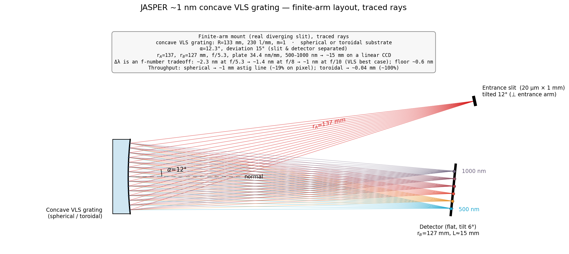
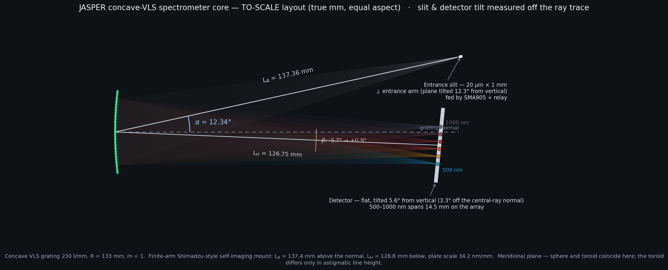
Grating: 230 l/mm, incidence ~12°, arms ~137 / 127 mm, R = 133 mm.
Plate scale: 34.2 nm/mm.
Detector: 500–1000 nm disperses across ~15 mm — sits on any linear CCD ≥15 mm; a $10 TCD1304 (29 mm, 3648 × 8 µm) covers it with room to spare. The same grating reaches ~400–1100 nm (~20 mm) if you want the wider NIR range.
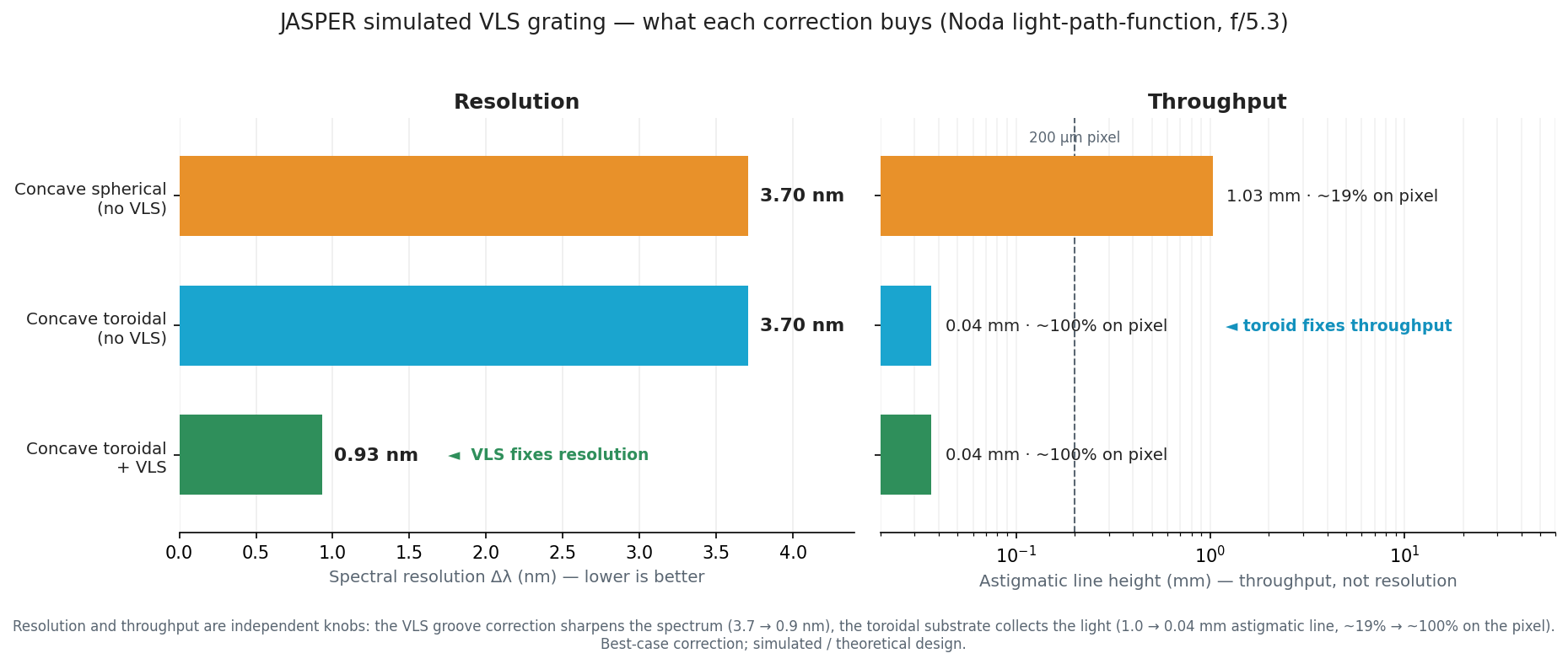
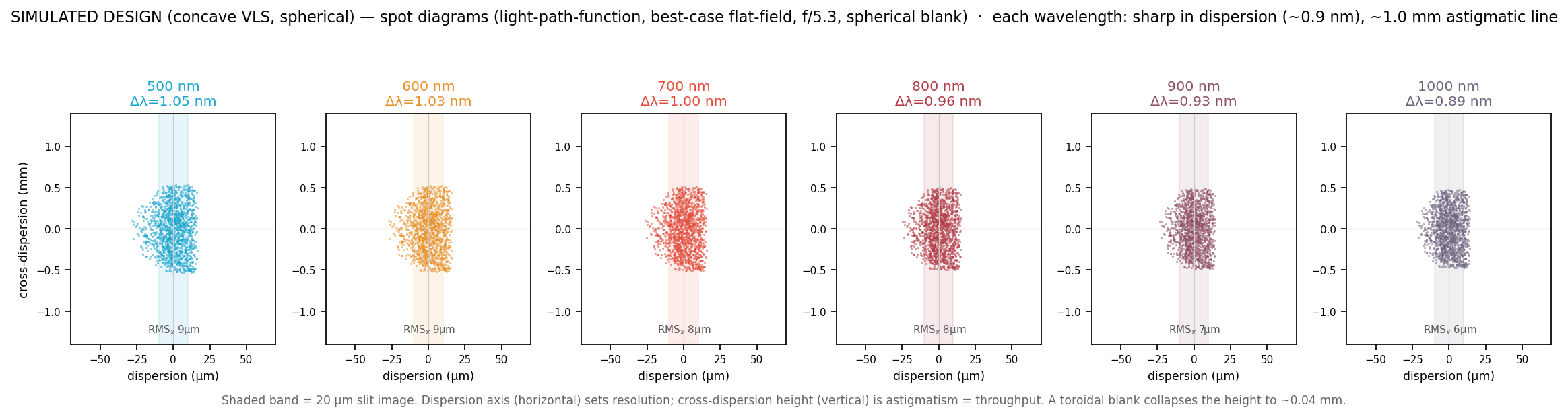
Substrate — spherical vs toroidal:same resolution, but the toroid collapses the astigmatic line and boosts throughput ~25× (a throughput upgrade, not a resolution one).
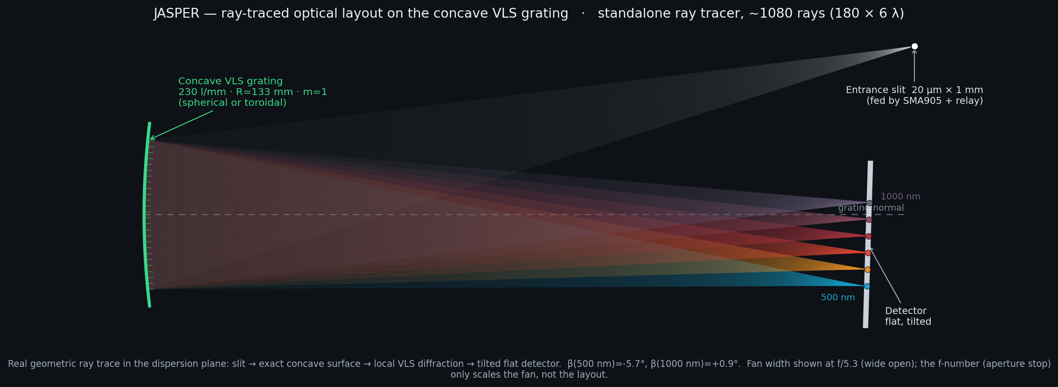
FIGURE: the optical core, real ray-traced (slit → concave surface → local VLS diffraction → tilted CCD), not a schematic
Resolution is an f-number tradeoff — not a single spec
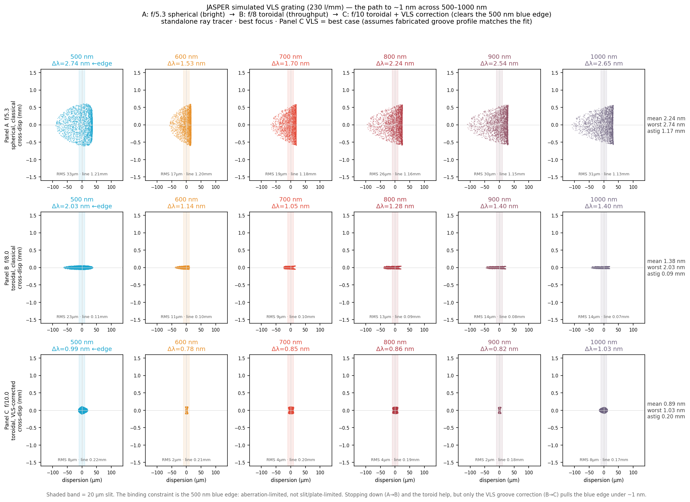
The headline is a curve, not a number. Faster f = more light but more aberration; slower f + the VLS groove correction = sharper. Ray-traced across 500–1000 nm, three points along the path:
working point
mean Δλ
500 nm edge
f/5.3 spherical (wide open)
~2.2 nm
~2.7 nm
f/8 toroidal
~1.4 nm
~2.0 nm
f/10 toroidal + VLS correction (best case)
~0.9 nm
~1.0 nm
floor (slit + pixel + diffraction)
~0.6 nm
—
Takeaway: hitting ~1 nm across the band needs all three knobs together — stop down to ~f/10, use the toroid for throughput, and apply the VLS groove correction. None alone is enough. And the binding constraint is the 500 nm blue edge, which is aberration-limited (not slit-limited) — it's the last thing to come down.
On "best case": the ~0.9 nm assumes the fabricated groove correction matches the design. The uncorrected classical grooves are the guaranteed floor; the VLS number is the plausible target a real aberration-corrected grating is built to hit. We're posting all, for a fair comparison.
FIGURE: the f/5.3 → f/8 → f/10+VLS path to ~1 nm, real ray-traced spots
FIGURE: what each correction buys: the VLS grooves fix resolution (3.7 → 0.9 nm), the toroidal substrate fixes throughput (astigmatic line 1.0 → 0.04 mm). Two independent knobs, not alternatives.
Modeled two ways
We checked the design twice:
Analytic — Noda–Namioka light-path-function theory (grating equation → dispersion; aberration coefficients → spot sizes from the mount geometry).
Ray trace — our own standalone NumPy tracer, real rays through the exact surface with the local VLS equation.
They match exactly on dispersion and astigmatism. On resolution they diverge slightly — the ray trace captures higher-order aberration the 3rd-order analytic theory truncates — which is why the honest number is the f-number curve, not the analytic floor alone. (A tooling note: we started in Optiland but it couldn't hold dispersion and focus at once for this off-axis reflective mount; Beam4 can't model variable line spacing at all — so we wrote our own tracer, which also draws the ray-fan layouts. All code in the repo, retired experiments marked.)
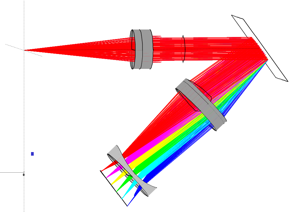
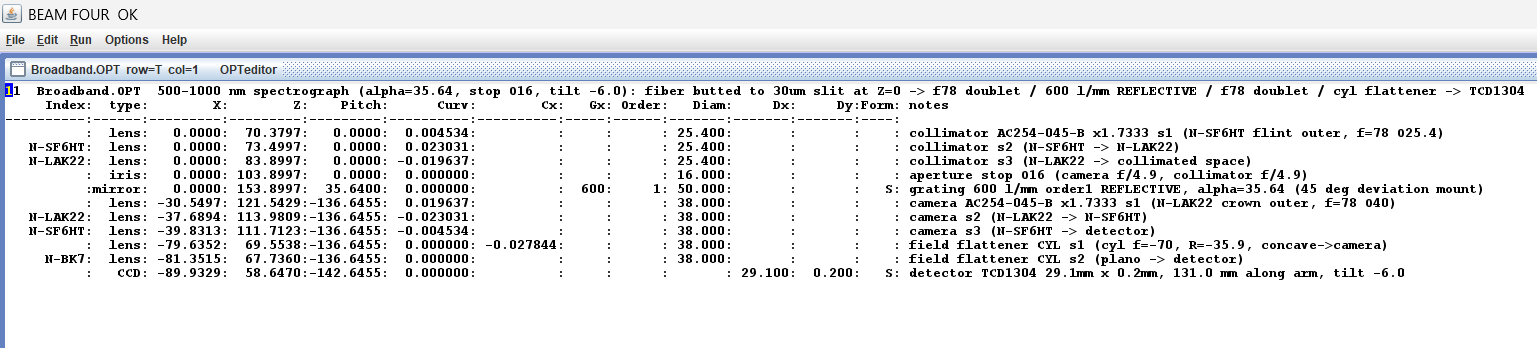
Optical ray trace: (two formats, and pick which one you like)
What's next
Phase 2: the buildable side. Coupling a standard SMA fiber to the slit, and a real catalog grating (Shimadzu P0400-01, whose full mount is published) with the same f-number resolution story. Spoiler: the relay sets throughput, not resolution — the slit sets the line width.
Last time we shared a 500–1000 nm spectrometer design that landed around 3–4 nm resolution. Decent, but not great — best was 2.1 nm at 600 nm, worst stretched to 4.2 nm. We suspected the camera was holding us back. Turns out we were right, and the fix came from a lens that’s curved in only one direction. With it, the design now sits at ~1.9 nm across the band, confirmed in BeamFour. And as always, it’s open‑source
Where we left off
Our earlier log traced a cost-optimised 500–1000 nm spectrometer built from stock 1‑inch lenses. It worked, but the resolution sat around 3–4 nm and the spots got fat toward the edges of the band. We said at the time that the limit wasn't the colours and wasn't diffraction — it was something about the camera. This log is what that "something" turned out to be, and how we fixed it.
Everything here is done in BeamFour, a free ray tracer, plus a few Python scripts. No expensive optics software.
The problem: the camera focuses onto a bowl, not a flat plane
When we looked carefully, every wavelength was actually sharp — at its own best focus. The catch is that "best focus" isn't at the same distance for every colour. It swings back and forth by about 2 mm across the band, in a smooth curve. The camera's focal surface is a shallow bowl, and our detector is flat, so only part of the spectrum can ever be in focus at once. The band edges (500 and 1000 nm) sit deepest in the bowl, which is exactly where the spots were worst.
This is called field curvature, and it's a property of a simple lens — not colour, not diffraction. Tilting the detector helps a little (it lines up with the average slope), but you can't tilt a flat plane to match a curved bowl.
The fix: a lens curved in only one direction
Here's the key insight. In a spectrometer, only one axis matters for resolution — the direction the colours spread out in (the "dispersion axis"). Blur in the other direction (along the slit height) just smears the line vertically; it doesn't mix one wavelength into the next.
So instead of a normal (spherical) corrector lens, we used a cylindrical one — a lens curved in the dispersion plane and flat in the other. It flattens the focal bowl exactly where it counts, and leaves the slit-height axis alone. A normal spherical corrector would also stretch the whole spectrum (it acts like a Barlow) and we'd run off the end of the sensor; the cylinder sidesteps that because it only has power in the one plane.
It's a plano-cylindrical piece of N‑BK7, sitting just in front of the detector.
Figure 1: The full trace. Fiber (far left) → collimator → grating → camera → the cylindrical field flattener (the small concave lens before the detector) → TCD1304. The rainbow is the 500–1000 nm spectrum being sorted onto the sensor.
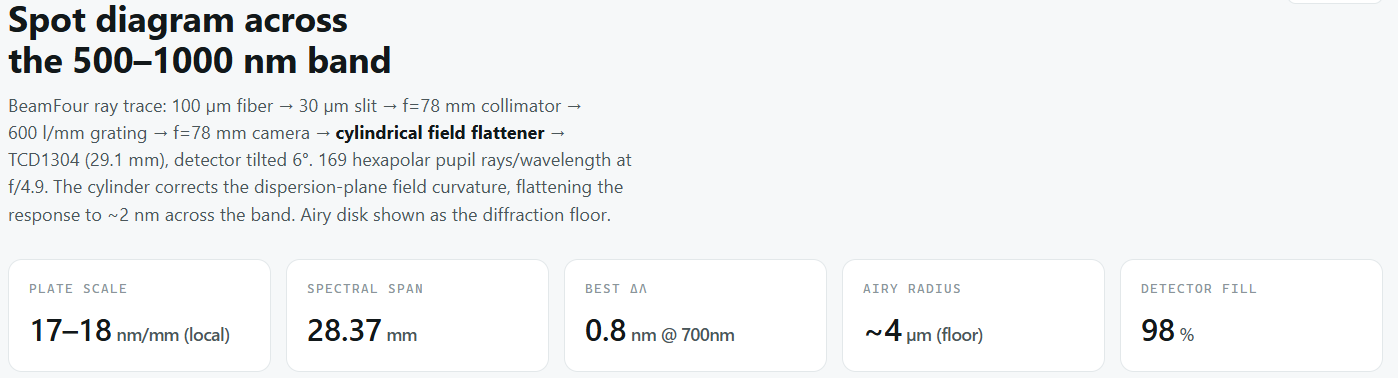
The result: ~1.9 nm
With the cylinder in and the detector refocused, the delivered resolution across 500–1000 nm is:
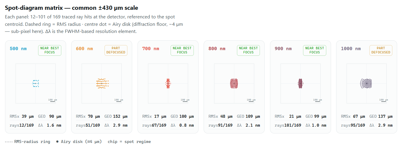
~1.9 nm mean, 2.9 nm worst (single exposure)
every wavelength between about 0.8 and 2.9 nm — no bad outlier
That's roughly a 40% improvement on where we were. And this number isn't just from our own script: we encoded the cylinder in BeamFour's own format and traced it there. Our offline tracer and BeamFour agree to better than a tenth of a micron on every wavelength, so the physics is trustworthy.
Figure 2:The spot analysis from the BeamFour trace. Each panel is one wavelength; the numbers are the RMS spot size and the delivered resolution Δλ
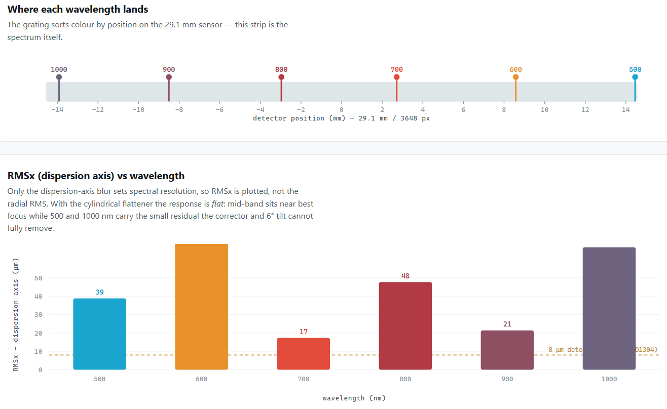
Figure 3: RMSx (spectral-axis blur) for each wavelength. The dashed line is one detector pixel.
Two Points worth noting
We removed the fiber relay entirely. The old design imaged the fiber onto the slit through a pair of lenses; a commenter on our last post rightly pointed out that (a) those relay aberrations don't actually belong in the spectrometer's resolution budget, and (b) for a fiber instrument you can just butt the fiber right up to the slit. That's what we do now — the fiber sits at the slit plane, a 100 µm fiber overfilling a 30 µm slit, which also keeps the wavelength calibration stable if the alignment drifts. Fewer parts, cleaner model.
And the flattener is a custom part — like our scaled f/78 doublet, it's not a catalogue item, so it has to be made.
What it would take to reach 1 nm
For anyone curious how much further this could go: each wavelength is already ~0.5 nm at its own best focus, so the optics themselves aren't the wall — the single flat detector is. The remaining error is the small chromatic part of the focal curve that one cylinder can't fully remove. Closing that to a genuine single-shot ~1 nm would take a field-corrected, multi-element camera (a Petzval-type group with enough degrees of freedom for the full field), which is a real optical-design job rather than a part swap. We haven't taken that on — the ~1.9 nm above is the design we're actually putting forward.
It's all open
Design files, the Python scripts, and a step-by-step to reproduce the exact 1.9 nm result in BeamFour are on our GitHub. Everything lives in one folder, python frontend_gen.py with no arguments regenerates the design, and there's a reference trace to check yours against. Code is MIT; the optical design is CERN‑OHL‑S.
Before building the hardware, the design should be simulated. Ideally, we would like to have a spectrometer design covering 400-1000nm, but cleanly covering the full 400–1000 nm needs a more complex (and costly) order-sorting filter, which goes against our aim of an affordable, user-modifiable instrument. This log covers a cost-optimised design: a budget design for 500–1000 nm built entirely from 1‑inch off‑the‑shelf lenses and a short Hamamatsu linear detector. The challenge: how much performance can you squeeze out of affordable, standard parts?
The optic design uses BeamFour, a free ray‑tracer, plus small Python scripts to derive the spot size. No expensive optics software needed.
We will walk through the design, then explain every parameter we use to judge it, so the charts further down make sense even if you've never touched optics software.
The design
Light comes in from an optical fiber, gets collimated (turned into a parallel beam) and re-imaged 1:1 onto a narrow entrance slit. That slit is the "object" the spectrometer looks at. After the slit, a lens collimates the light again and sends it onto a diffraction grating, which is the part that actually splits broadband light into its colours by bending each wavelength through a slightly different angle. A final camera lens focuses each colour to its own spot on the detector. Because different colours land at different positions, the detector sees the spectrum — a strip of light where position equals wavelength.
It's called a 4f design because the lenses are spaced by their focal lengths in a way that keeps the beam well-behaved, and it's folded (bent with the grating and layout) so the whole thing fits in a small box.
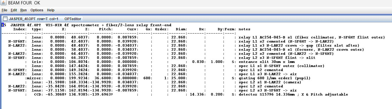
Figure 1: The JASPER 4f prescription in BeamFour. Each row is one optical surface — the four doublets, the 30 µm slit, the 600 l/mm grating, and the tilted S15796 detector.
This is the actual "recipe" for the instrument, as BeamFour stores it. Each line is one optical surface — one face of a lens, the slit, the grating, or the detector — described by where it sits and how strongly it's curved. Reading it top to bottom follows the light:
Four identical doublets (AC254-045-B). A doublet is a lens made of two glasses cemented together (here a crown glass, N-LAK22, and a flint glass, N-SF6HT). Gluing two glasses together cancels most of the colour smear a single lens would add. All four lenses in the system are the same stock 45 mm, 1-inch Thorlabs part — that's the "cost-optimised" part of the story. Two form the fiber relay, one is the collimator, one is the camera.
The 30 µm entrance slit. Listed as the iris, 0.030 mm wide.
The grating, 600 lines per mm, working in first order — the disperser.
The detector (CCD), a Hamamatsu S15796, 14.336 mm long, whose position and tilt we're allowed to adjust.
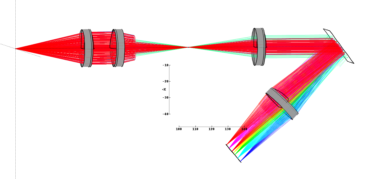
Figure 2: BeamFour ray trace of the full folded path: fiber → 1:1 relay → slit → collimator → grating → camera lens → tilted detector. The colours fanning out at bottom right are the 500–1000 nm spectrum being sorted onto the sensor.
This is what a ray trace looks like: the software fires hundreds of light rays through the design and draws where each one goes. On the left, the fiber light is relayed to the slit (the pinch point in the middle). It's then collimated, hits the grating, and the camera lens (lower right) focuses it down.
The rainbow fan at the bottom right is the whole trick of a spectrometer made visible — the grating has bent each colour by a slightly different angle, so red, green and blue rays arrive at different places on the detector. That spread along the detector is the spectrum.
How we judge the design — the parameters:
Before the analysis charts, here's what each number means. Every one of these is measured from the traced rays.
Spot / spot diagram. When the camera focuses one single colour, it should ideally land as one perfect point. In reality it lands as a small smudge of rays called a spot. A spot diagram is just a zoomed-in picture of where all the rays for one colour actually hit. Smaller, tighter spot = sharper instrument.
Centroid. The average position of all the rays in a spot — i.e. the "middle" of the smudge. For the dispersion direction, the centroid is where that colour's spectral line effectively sits on the detector.
RMSx — the number that sets resolution. RMS stands for root-mean-square, which is just a careful way of saying "typical spread." RMSx measures how far the rays are spread out along the direction colours are separated (the dispersion axis). We only care about this direction, because spreading sideways doesn't blur one colour into the next — only spreading along the colour axis does. In one line: RMSx = √⟨(x − centroid)²⟩, converted to microns. Smaller RMSx = a sharper spectral line.
GEO — the worst-case spot size. Where RMSx describes the typical spread, GEO (geometric radius) is the distance from the centroid to the single farthest ray in the spot. It's the full footprint — the circle that contains every ray. It's always bigger than RMSx and is driven by the most poorly-behaved ray at the edge of the beam. We report it as a reality check on how large the spot can get.
Airy disk / diffraction floor. Physics says no lens can ever focus light to a perfect point — diffraction spreads it into a tiny blob called the Airy disk. Its size is fixed by the wavelength and the lens speed (about 2 µm here). This is the best case: no design can beat it. In our spots it shows as a tiny centre dot. Because our real spots are 10–40× larger than this dot, the design is geometry-limited — meaning lens imperfections, not diffraction, are what set the blur. (BeamFour is a geometric tracer, so it can't model diffraction directly; we draw the Airy disk in as an analytic reference, using the standard formula 1.22 × wavelength × f-number.)
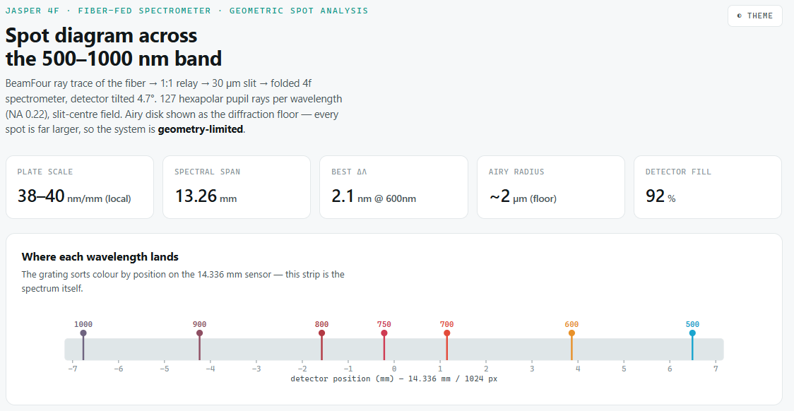
Dispersion scale (nm/mm). How many nanometres of spectrum are packed into one millimetre of detector. Here it's 38–40 nm/mm. Lower would mean the colours are spread out more (finer detail); higher means they're squeezed together. It's not constant across the band, so we always measure it locally from the traced spots rather than using one average.
Spectral span. The total length the whole 500–1000 nm spectrum occupies on the sensor — 13.26 mm here.
Detector fill. What fraction of the sensor's length the spectrum actually uses. 92% means we're filling almost the whole 14.336 mm sensor — good, because unused sensor is wasted resolution.
Δλ (delta-lambda) — the delivered resolution. This is the bottom-line number: the smallest wavelength difference the instrument can actually distinguish, in nanometres. Smaller is better. It's built by combining the three things that blur a spectral line, added in "quadrature" (square them, add, square-root — the right way to combine independent blurs):
slit image — the finite width of the slit projected onto the detector (30 µm, slightly narrowed by geometry),
2.355 × RMSx — the optical blur. The 2.355 converts the RMS spread into a FWHM (full-width-at-half-maximum), which is the ideal way to state a line width,
pixel — the detector's 14 µm pixel, which can't resolve anything finer than itself.
rays n / 127 — survivors vs launched. For each colour we launch 127 rays arranged in a pattern across the beam. Some get clipped by the edges of lenses or apertures on the way through (this is called vignetting). The n / 127 count tells you how many survived to reach the detector. A lower number means more of that colour's light is being lost, so its measured spot rests on fewer rays.
Figure 3: Top-level results. The five tiles summarise the whole design; the strip below shows exactly where each wavelength lands on the 14.336 mm sensor — that strip is the spectrum itself.
The five tiles are the headline numbers, now that you know what they mean: dispersion scale 38–40 nm/mm, the spectrum spanning 13.26 mm, a best-case resolution of 2.1 nm (at 600 nm), the ~2 µm diffraction floor, and 92% of the sensor used.
The strip underneath is the most intuitive picture in the whole analysis: it's the sensor drawn to scale, with a coloured tick showing where each wavelength actually focuses. This is, quite literally, the spectrum the instrument would produce.
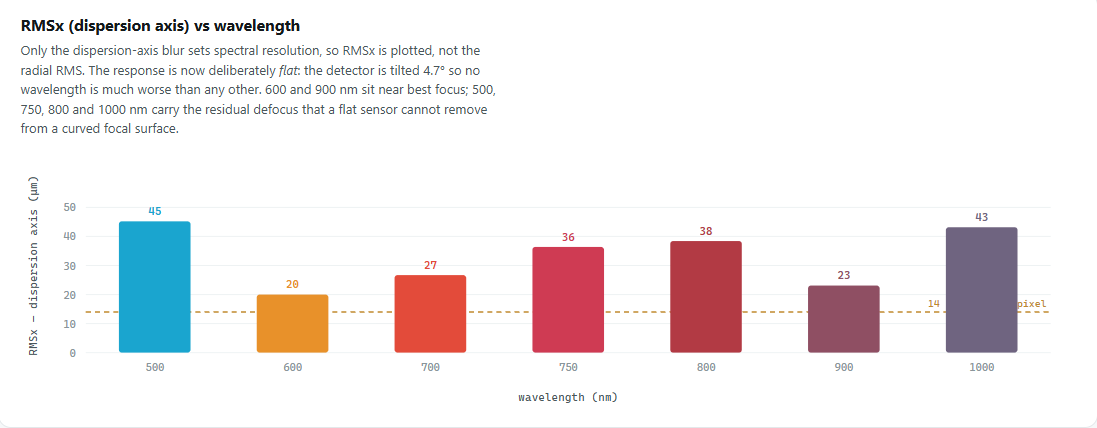
Figure 4: RMSx (spectral-axis blur) for each wavelength. The dashed line is one detector pixel. The response is deliberately flat — no wavelength is far worse than the others.
This bar chart shows RMSx at each wavelength. The interesting thing isn't any single bar — it's that they're all roughly similar height. That flatness is on purpose. 600 and 900 nm sit near best focus (sharpest); 500, 750, 800 and 1000 nm carry a bit of leftover blur. But nothing is catastrophically bad, which is exactly what you want in a spectrometer that has to work across the whole band, not just in the middle.
The dashed line marks one 14 µm pixel, so you can see the blur in units of "how many pixels wide is this."
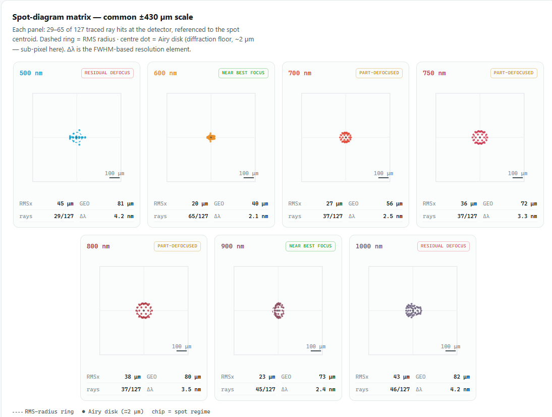
Figure 5: One spot per wavelength, all drawn to the same ±430 µm scale. Dashed ring = RMS radius, centre dot = the ~2 µm Airy disk. The small print under each panel gives RMSx, GEO, the surviving ray count, and Δλ.
Now you can read every panel. Each shows the actual cloud of surviving rays for one colour, all on the same scale so they're comparable. The tiny centre dot is the diffraction floor (the best any optics could do); the fact that every real spot dwarfs it is the visual proof that we're geometry-limited. Under each panel are the four numbers we defined: RMSx, GEO, rays-survived, and Δλ.
Notice the shapes differ — some are tight blobs, some are little rings or arcs. Those shapes are the fingerprints of specific lens aberrations, which leads to the one genuinely surprising result.
The surprise: it's not the colours, it's the curved focus
The obvious guess for why the band edges (500 and 1000 nm) are softer than the middle is chromatic aberration — the classic problem where a lens focuses different colours at slightly different distances. It's the intuitive villain.
But when we isolated the camera lens and tested it two ways, the data said otherwise:
Hold the colour fixed and only change the angle the light enters at (which is what really changes as you move across the band): best focus moved by about 2.3 mm. This is field curvature — the lens focuses onto a gently curved bowl-shaped surface, not a flat plane, so off-centre colours focus at a slightly different depth.
Hold the angle fixed and sweep the colour across the whole 500–1000 nm range: best focus moved only about 0.37 mm. That's the actual chromatic effect — and it's tiny.
So the real limiter is field curvature, about six times bigger than the colour effect. The doublets are doing their job on colour; it's the flat sensor trying to catch a curved focus that costs us sharpness.
That's also why the detector is tilted 4.7°. A tilt can't un-bend a curved focal surface, but it can line the sensor up as well as possible with it — trading a little sharpness in the middle to rescue the ends. It's why the RMSx chart is flat rather than pointy.
The ceiling
There's a hard limit hiding in the geometry. Squeezing 500 nm of spectrum onto a 14.336 mm sensor forces about 37–40 nm/mm, and once you fold in the pixel size, the finest resolution this sensor can ever deliver is around 1 nm — no matter how perfect the glass is. We're already within about 3× of that wall.
So the biggest single upgrade isn't fancier lenses — it's a longer detector. A 29.1 mm sensor would roughly halve the dispersion scale and unlock the resolution the optics are capable of. That's the next move.
Why this approach
The whole point of doing this in BeamFour plus Python — rather than a costly commercial tool — is that it's reproducible and free. We even wrote a small Python tracer that reproduces BeamFour's output exactly, so we can scan hundreds of "what if we tilt the detector 0.1° more?" variations offline in seconds, then confirm the winner with a real BeamFour trace. BeamFour stays the authority; Python just makes the search fast.
If you're building a spectrometer on a budget, the takeaway is that stock 1-inch doublets and a free ray tracer get you to a genuinely useful VIS–NIR instrument — and that reading the spots carefully tells you exactly which part to spend your next rupee/dollar on. For us, that's the detector, not the lenses.
Quick glossary
Spot — the little smudge of rays one colour actually focuses to (ideally a point).
Centroid — the average/centre position of a spot.
RMSx — typical spread of the spot along the colour axis; sets resolution. Smaller = sharper.
GEO — distance to the farthest ray; the worst-case spot size.
Airy disk — the ~2 µm diffraction limit; the smallest spot physics allows.
Geometry-limited — spots are far bigger than the Airy disk, so lens shape (not diffraction) sets the blur.
Plate scale — nanometres of spectrum per millimetre of detector (38–40 nm/mm here).
Spectral span — how long the full spectrum is on the sensor (13.26 mm).
Detector fill — fraction of the sensor used (92%).
Δλ — the delivered resolution: smallest wavelength gap the instrument can separate.
FWHM — full-width-at-half-maximum, the honest width of a blurred line (= 2.355 × RMS).
Vignetting — rays clipped by lens/aperture edges; why not all 127 launched rays survive.
Field curvature — the lens focuses onto a curved bowl, not a flat plane — our real limiter.
4f / folded — a compact lens spacing, bent to fit in a small enclosure.
Most VIS-NIR spectrometers designed for specific applications require fine customization of spectral span, optical resolution, or Signal-to-Noise Ratio (SNR).
For instance, the Zemax spectrometer design guide highlights a system tailored for Optical Coherence Tomography (OCT) in retinal imaging. That specific application demands a narrow 50nm bandwidth (855 nm to 905 nm) optimized for deep, non-invasive imaging within the near-infrared biological window.
However, standard optical simulation software (such as Ansys Zemax OpticStudio) often falls short when modeling physical diffraction efficiency curves, real-world blaze angles, and practical mounting tolerances. For researchers, optical engineers, and hardware builders, having a physical, reconfigurable benchtop setup is indispensable.
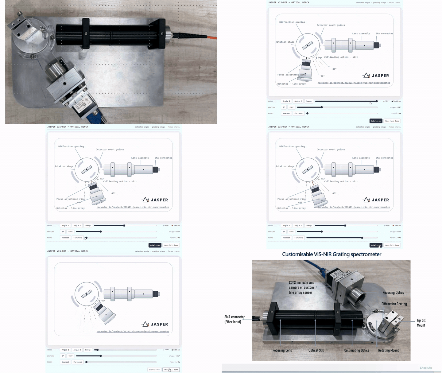
We are building a truly customizable, open-source optical benchtop for reflective-grating spectrometers that allows you to easily swap and tune key hardware parameters:
Slit Sizing: Interchangeable mechanical slits to balance optical throughput against spectral resolution.
Optics Selection: Modular lens mounts to evaluate different collimating and focusing focal lengths.
Grating Geometry: Independently adjustable incident (α) and diffracted (β) angles to test custom blaze conditions and spectral dispersion profiles.
Sensor Versatility: Flexible detector positioning to evaluate COTS camera modules or specialized high-speed linear CCD/CMOS array sensors.
To help refine the optical layout and clear aperture tolerances for the JASPER VIS-NIR Spectrometer, we built a lightweight, interactive simulator that models our optical bench mechanics directly in the browser!
When designing compact Czerny-Turner or transmission-grating VIS-NIR optical benches, balancing detector arm placement against grating rotation is always a trade-off between spectral range and focus depth.
This simulator lets you interactively adjust and test:
Detector Angle (Φ): Sweep the detector arm continuously from 45° to 95°across reference markers to see the central wavelength (λ) shift across the line array.
Grating Rotation Stage: Rotate the primary diffraction grating stage (0° to 50°) independently of the detector arm.
Focus Travel Calibration: Slide the sensor along its own optical axis (0% to 100% travel) to evaluate focal distance tweaks relative to the focusing optics.
Real-time Ray Tracing: Visualizes how the diffracted spectral band maps across the active sensor plane.
Built for Open-Source Transparency
Rather than relying on heavy desktop CAD packages or proprietary optical simulation software for quick spatial checks, we built this tool with pure, self-contained HTML5, CSS, and inline SVG. It requires zero external assets or dependencies, making it instantly scannable and accessible on desktop or mobile.
Feel free to run the "Run full demo" loop on the page to see the automated mechanical sweep sequence in action, or turn off labels for a clean visual view!
The repository is fully open-source under the MIT license:
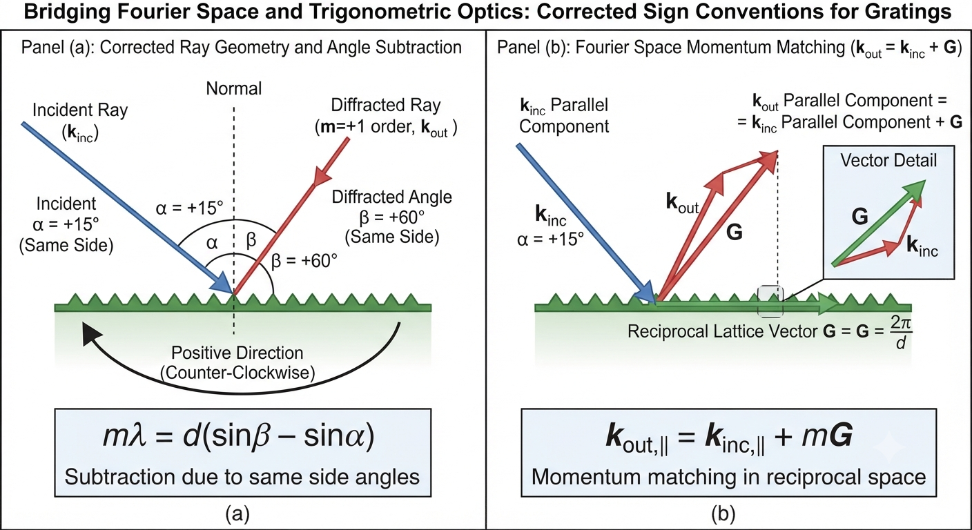
It all started with a diagram in the JASPER project logs that didn't quite look right. The angle subtraction geometry for the diffraction grating felt ambiguous, leading to a rabbit hole of second-guessing and a quick post over on Reddit to see if the community could untangle it. A helpful comment pointed toward a deeper truth: if you really want to understand gratings, stop thinking purely in right triangles and start looking at them from Fourier space.
That advice sparked a dive into reciprocal lattices, Bloch waves, and vector formulations. But rather than just taking someone's word that "vector mechanics and trigonometry are the same thing," let’s build the actual bridge between them.
The Diagram That Started It All
When dealing with real-world layouts, getting the sign conventions right for angle subtraction matters immensely. If your angles are on the same side of the normal, you subtract them; if they're on opposite sides, you add them. But why does the math behave this way? To find out, we have to look at the boundary through the lens of electrodynamics.
The Fourier Space Perspective: Bloch Waves and Momentum Matching
Periodic structures—whether an array of micro-grooves or nanophotonics particles—impose discrete spatial periodicities. From a rigorous standpoint, every electromagnetic field interacting with a periodic grating must obey Bloch's theorem. When you expand the grating's spatial profile into a Fourier series, periodicity naturally translates into discrete momentum contributions in reciprocal space. In wavevector terms, the parallel component of the outgoing wavevector isn't arbitrary; it is shifted by a discrete reciprocal lattice vector
:
This component-based formulation
is fundamentally the exact same concept as the classical grating equation, expressed as momentum conservation.
The 2-Line Bridge: From Fourier Space to Trigonometry
For a Hackaday audience, equations are best when you can trace them back to something you can plug into a spreadsheet. Let's look at the x-components of our wavevectors in 1D to see how Fourier space collapses back into the classic formula.
Start with the reciprocal lattice condition:
Substitute the wavevector magnitudes
in terms of angles relative to the normal
and the grating period
results in
Divide the entire expression by 2*pi / λ and rearrange, and you arrive right back at the familiar form:
Just like that, abstract Fourier-space momentum matching resolves cleanly into the trigonometry we use on the benchtop.
Practical Takeaways for Spectrometer Design (e.g., JASPER)
1. When to use trigonometry: For a standard 1D VIS-NIR spectrometer layout where light stays strictly in-plane (perpendicular to the grooves), the classical equation
is efficient and accurate. Handling angle subtraction properly keeps your layout geometry straightforward.
2. When vector mechanics matter: If you move away from simple in-plane designs into conical diffraction geometries (out-of-plane scattering), or if you need to calculate rigorous diffraction efficiencies and polarization-dependent behaviors, the full vector/reciprocal lattice approach becomes essential.
By connecting the confusing diagram on the wiki to a Reddit thread, and a Reddit thread to Fourier-space electrodynamics, we’ve closed the loop. Good optics isn't just about plugging numbers into formulas—it's about knowing why the formulas work when the diagrams start looking weird.
When designing a grating-based spectrometer, the primary challenge is not solving the physics—it's managing the real-world constraints of Commercial Off-The-Shelf (COTS) components. We must design around fixed detector lengths (LD) and standard focal lengths (LF).
This presents a chicken-and-egg problem: finding the right Grating Groove Density (G) without first committing to a fixed Focusing Lens Focal Length (LF). We can get an early estimate for G based only on the desired Wavelength Span and the Geometry of our optical setup.
The Core Design Principle: The Grating Equation Governs G
The fundamental constraint is that the total angle the dispersed light occupies (∆β) must be related to the total wavelength span(∆λ). This relationship is governed purely by the Grating Equation, independent of any focusing optics.
Step 1: Grating Equation for the Span Edges
The Grating Equation (for the first order, m=1) relates wavelength (λ), angles (α, β), and groove density (G):
By setting up this equation for our minimum (λmin) and maximum (λmax) wavelengths, and assuming the Angle of Incidence (α) is constant:
Step 2: Isolating G
Subtracting the first equation from the second elegantly removes the α term:
By rearranging, we get the key design relationship for G:
3. The Early Estimate: Setting a Practical Angular Window (∆β)
A COTS detector array can typically only capture light over a limited angular span (∆β), usually between 30° and 50°. By defining a center angle (βcenter) and a total angular span (∆β = βmax – βmin}), we can simplify the numerator using a trigonometric identity:
This gives us the final, actionable equation for estimating the required groove density:
Let's assume a full VIS-NIR span (∆λspan = 650nm) and a Center Angle βcenter = 15°.
Angular Span (∆β)
Trig Difference (∆sinβ)
Required Gestimate (lines/mm)
COTS Choice
30°
0.50
769
600 or 1200
40°
0.64
985
1200
50°
0.79
1215
1200
Conclusion: Making the COTS Decision
This early estimate methodology shows that for a wide VIS-NIR span, a 1200 lines/mm grating is the most likely candidate. Once G is fixed by this COTS selection, we can move to the next critical step: using the chosen G along with the fixed detector size (LD}) to calculate the exact required Focal Length (LF) for the focusing lens. This ensures the physical design is robust and uses readily available components.
When designing a spectrometer, every photon counts! You can buy the fanciest grating in the world, but if your collimator mirror or lens is shining light past it, you're throwing away precious signal.
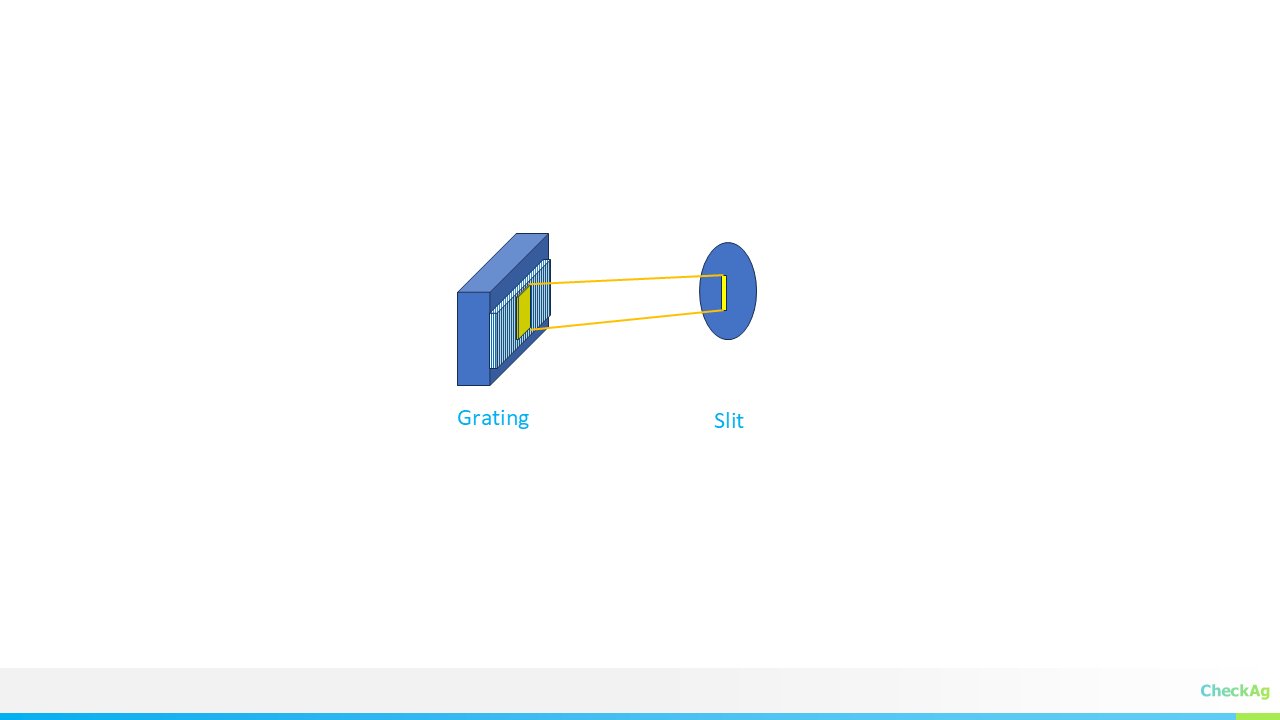
The key to a high-efficiency spectrometer is ensuring your grating is wide enough to capture the entire cone of light emitted from your input slit or fiber. This isn't just the beam diameter—it's the beam diameter plus a correction for the angle at which the light hits the grating.
Here’s the step-by-step derivation to find the absolute minimum physical width required for your diffraction grating Wgrating
Step 1: Defining the Light Cone and the Collimated Beam
The light exiting your input source (fiber or slit) spreads out in a cone defined by its Numerical Aperture (NA).
Numerical Aperture (NA): This value is usually provided for optical fibers. If you have a slit and a lens, you calculate the NA from the lens-slit geometry.
Where θNA is the half-angle of the light cone.
Collimator Focal Length (Lc): The light cone hits the collimator mirror or lens at a distance Lc. The collimator converts this diverging light cone into a parallel beam.
The maximum radius (R) of the light cone at the collimator mirror, and thus the radius of the resulting parallel beam, is found using basic trigonometry:
The total beam diameter (Dbeam) is simply twice the radius:
Step 2: The Grating Tilt—Why Wgrating > Dbeam
If your grating were positioned perfectly perpendicular to the incoming beam (α= 0°), then your required grating width (Wgrating) would simply equal the beam diameter (Dbeam).
However, in virtually every spectrometer design (like Czerny-Turner or Littrow), the grating is tilted by the angle of incidence, α.
Because the grating is tilted, the parallel beam's cross-section is stretched when projected onto the grating's surface. Think of a spotlight hitting a wall at an angle—the illuminated area is larger than the spotlight head.
The relationship between the true beam diameter (measured perpendicular to the light path) and the required physical width of the grating (measured along its surface) is given by:
Rearranging this, we find the Cos(α) Correction Factor:
Step 3: The Final, Practical Grating Width Formula
We now substitute the expression for Dbeam from Step 1 into the equation from Step 2 to get the complete, actionable formula for the minimum required grating width:
Since the half-angle θNA is defined by the Numerical Aperture,
the final formula is:
Practical Implications for Design
NA is a Killer: If your fiber has a high NA (e.g., 0.22), the
term grows quickly, requiring a much wider grating or a much longer focal length Lc.
Angle of Incidence Matters: The higher your angle of incidence (α) is (e.g., 60° for high dispersion), the smaller cos(α) becomes, meaning Wgrating gets much larger. This is why high-dispersion designs often require the largest and most expensive gratings!
Use this formula early in your design process to balance cost, size Lc, and efficiency.
After struggling to design a spectrometer in Czerny turner configuration using spectrometer design guide https://ibsen.com/resources/spectrometer-resources/spectrometer-design-guide/) and tool provided by Ibsen Photonics (https://ibsen.com/wp-content/uploads/Spectrometer.html), I uncovered a fundamental conflict between common spectrometer geometry and the raw physics of diffraction. This deep dive led to a surprising conclusion: for hobbyists and professionals building Czerny-Turner (CT) spectrometers, trying to calculate the Angle of Incidence (α) based on the fixed deviation angle (φ) is a recipe for failure with common high-resolution gratings.
The core issue? The seemingly simple inverse trigonometric functions, arcsin and arccos, impose severe, hidden limits on your choice of grating and wavelength.
The Grating Equation and the Two Geometries
The physics of diffraction is governed by the Grating Equation:
where:
G is the groove density (grooves/mm)
λ is the center wavelength
α is the Angle of Incidence (AOI)
β is the Angle of Diffraction (AOD)
The +/- sign depends on whether alpha and beta are on the same or opposite sides of the grating normal.
The confusion arises from how the total Deviation Angle (φ)—the fixed angle between your collimating and focusing optics—is defined:
1. The Littrow-like Geometry (The Ibsen Tool Approach)
In compact and highly optimized spectrometers (like Ibsen's), the system operates close to the Littrow condition (alpha is approximately beta). The total deviation angle phi is defined as the difference:
When this definition is combined with the grating equation (sin(α) + sin(β) = G*λ), the resulting formula for the Angle of Incidence (α) involves an arcsin function:
The Practical Advantage: For this formula to work, the argument of the arcsin must be <= 1. This sets the limitation: G*m*λ<= 2 * cos(φ/2). Since φ is typically small (30 degrees), cos(φ/2) is close to 1. For φ=30 degrees, this limit is G*λ<= 1.932, which is generous and accommodates almost any commercial grating (e.g., 1200 g/mm at 550 nm gives G*λ=0.66, which works perfectly). This is why the Ibsen tool is so practical for Littrow-like geometry
2. The Classic Czerny-Turner Geometry (φ = α + β)
In the traditional CT setup, both the input and output rays are on the same side of the Czerny-Turner axis, leading to the simple geometric sum: (φ = α + β)
When this is combined with the same side of normal grating equation (sin(α) + sin(β) = G*λ), the resulting formula for alpha involves an arccos function (derived by exploiting the trigonometric sum-to-product identity, as seen in this derivation log):
The Hidden Czerny-Turner Limitation
This arccos-based formula is where practical design collides with math. For the arccos to return a real angle, its argument must be <= 1. This yields a dramatically tighter limitation:
Let's look at the numbers for a very common fixed deviation angle, φ=30 degrees:
This means that for a φ=30 degrees CT spectrometer using the φ=α+β definition, the product of G and λ MUST NOT exceed 0.5176 mm
Why Your High-Resolution Grating Won't Work (The Real-World Test)
Consider common commercial gratings:
Grating (G)
Max G*λ Limit (0.5176 mm)
Max Center Wavelength (λ_max)
Practical Use
300 g/mm
0.5176 mm
1725 nm
Works well across VIS/NIR.
600 g/mm
0.5176 mm
862 nm
Works well for VIS/short NIR.
1200 g/mm
0.5176 mm
431 nm
Fails for visible light (550 nm)!
1800 g/mm
0.5176 mm
287 nm
Restricted to Deep UV.
If you attempt to design a φ=30 degrees Czerny-Turner spectrometer (where φ=α+β) using a 1200 g/mm grating to look at green light (550 nm), the required G*λ product is 0.66 mm. Since 0.66 is greater than the 0.5176 limit, the arccos formula fails, and no real angles α and β exist that satisfy both the grating equation and the geometric sum!
The Superior Design Strategy: Fixing α
If you are using a fixed-angle Czerny-Turner setup and high-density gratings, the failure of the inverse trig functions shows that you cannot treat α as the unknown.
The most practical design approach for a CT system is to fix α (Angle of Incidence) and then calculate β (Angle of Diffraction) directly using the simplest form of the grating equation.
1. Define α: Choose a reasonable AOI, typically 10 to 20 degrees for good performance (or even 0 degrees if possible, though that introduces aberrations).
2. Calculate β: For your center wavelength (λc), calculate the required diffraction angle
3. Check Geometry (φ): Now, calculate the actual deviation angle required by this combination:
4. Align Optics: Align collimating and focusing mirrors/lenses to match this φrequired
By adopting this strategy, you sidestep the fatal G*λ limitations of the arccos and arcsin formulas, allowing you to use high-resolution gratings with typical visible light while guaranteeing a real, physically implementable solution.
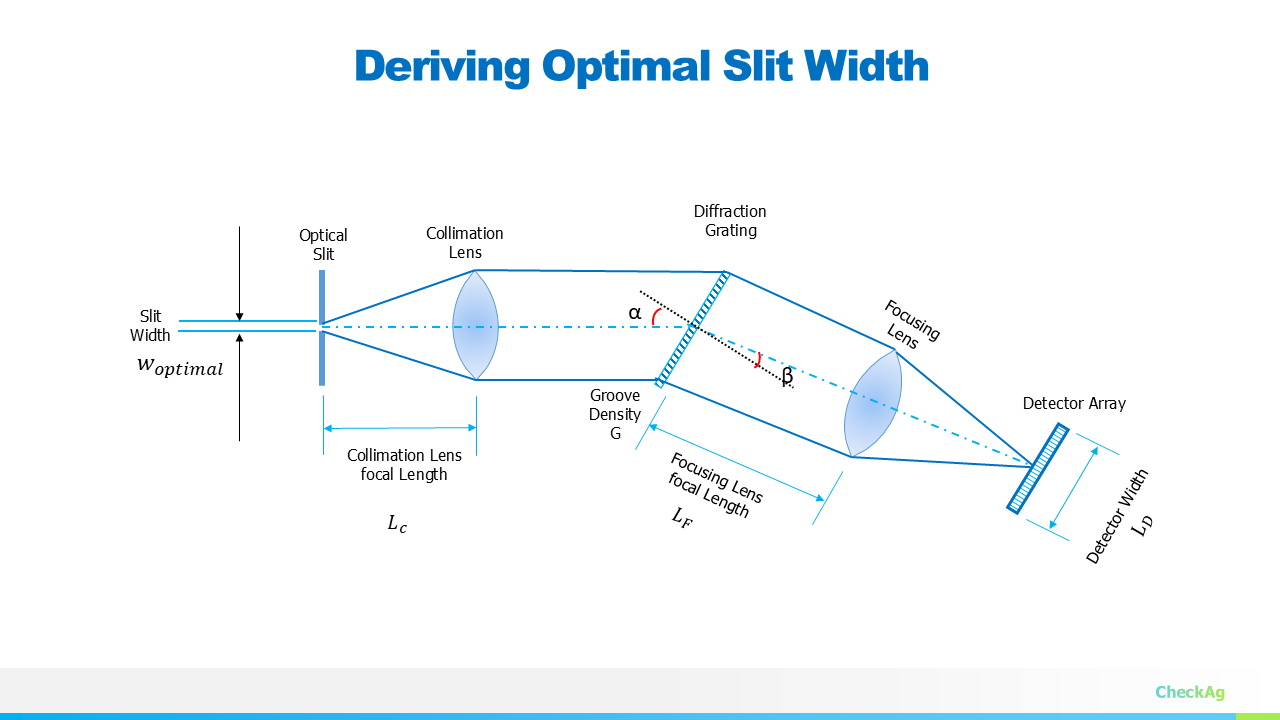
If you followed the theoretical deep dive in our last log,Spectrometer Design Part 8: Calculating Optimal Slit Width, you know that determining the entrance slit width (w) is the final, crucial step in the optical design of the JASPER spectrometer. This single parameter defines the fundamental trade-off: light throughput vs. spectral resolution.
To make setting this parameter effortless for any design, we're excited to announce the release of the interactive tool:
The JASPER VIS/NIR Optimal Slit Width Calculator
What the Tool Does
This online calculator instantly computes the ideal slit width based on your design goals, ensuring your system's resolution is perfectly matched to your detector's pixel size.
The calculator:
Explains the Math: It visually walks you through the four key steps (from the desired spectral resolution Δλ to the final equation) that were derived in the previous log.
Solves the Equation: It uses the final derived formula, which elegantly links the physical slit width to your core design parameters:
Where:
m = Diffraction Order
Δλ = Target Spectral Resolution
LC = Collimating Lens Focal Length
d = Grating Groove Spacing
β = Diffraction Angle
3. Provides an Interactive Interface: Just plug in your desired design values for spectral resolution, collimating lens focal length, grating grooves, and angle, and it instantly spits out the optimal slit width in micrometers (μm).
🖱️ Use the Calculator Now!
Whether you're building a JASPER or designing your own grating-based spectrometer, this tool will save you hours of manual calculation and help you lock in that perfect balance between light collection and spectrum clarity.
In our ongoing JASPER VIS-NIR spectrometer project, we have worked through the core components: fixing the geometry, selecting the grating, and deriving the focal lengths for the collimating (LC) and imaging (LF) lenses. The final piece of the optical puzzle is determining the optimal entrance slit width (w).
The slit width is critical because it directly controls the amount of light entering the system (the optical throughput) and also dictates the final spectral resolution. We need a slit that is wide enough to capture sufficient light but narrow enough not to degrade the resolution we designed the system for.
To find the optimal slit width, we must first recall the minimum required image size on our detector array.
Step 1: Minimum Resolvable Image Dimension (Δd)
The goal of any spectrometer is to distinctly separate two wavelengths that are very close to each other. This minimum difference in wavelength is our desired spectral resolution, Δλ.
For the spectrometer to register this change, the image of Δλ must be separated by at least two pixels on the sensor array. This means the minimum resolvable image dimension (Δd) must be equal to twice the pixel width.
The relationship between the change in wavelength (Δλ) and the resulting physical separation on the detector (Δd) is governed by the linear dispersion of the system:
LF is the focal length of the imaging (focusing) lens.
d is the grating groove spacing.
β is the angle of diffraction for the wavelength being resolved (often taken at λmin).
Solving for the smallest resolvable image dimension Δd at the desired spectral resolution Δλ:
For optimal performance, this dimension Δd should be set to match the physical requirement of the detector:
Step 2: Deriving the Optimal Slit Width (w)
In an infinity-corrected optical setup—where the collimating lens (LC) and the imaging lens (LF) are used—the slit width (w) is imaged onto the detector plane. The relationship between the object size (w) and the image size (Δd) is simply the ratio of the focal lengths of the two lenses:
We want the image of the slit to be exactly equal to our minimum resolvable image dimension (Δd) to ensure we utilize the maximum optical power without sacrificing resolution.
Now, we solve for the optimal slit width w:
Substituting the expression for Δd from Step 1 into this equation:
Notice that the focal length of the imaging lens,LF, cancels out, which significantly simplifies the final equation for the optimal slit width:
This final equation elegantly links the physical slit width to the core design parameters: the desired spectral resolution (Δλ), the grating characteristics (m and d), and the focal length of the collimating lens (LC). By setting the slit width according to this derivation, we achieve a system where the spectral resolution is perfectly matched to the detector's pixel size, thereby optimizing both light throughput and resolution.
In the next part, we will use all these derived equations to plug in our target values and finalize the physical dimensions of the JASPER spectrometer.
 Tony Francis