Project Logs

Collapse

• Rotating Magnets

  Ted Yapo • 01/13/2018 at 18:04 • 2 comments

  Someone on GitHub asked about using the MLX90393 to determine the angle of a permanent magnet.  I had to admit I had never tried to use this part for its presumably indented purpose.  So, after breakfast, I lashed some junk together to try it out.

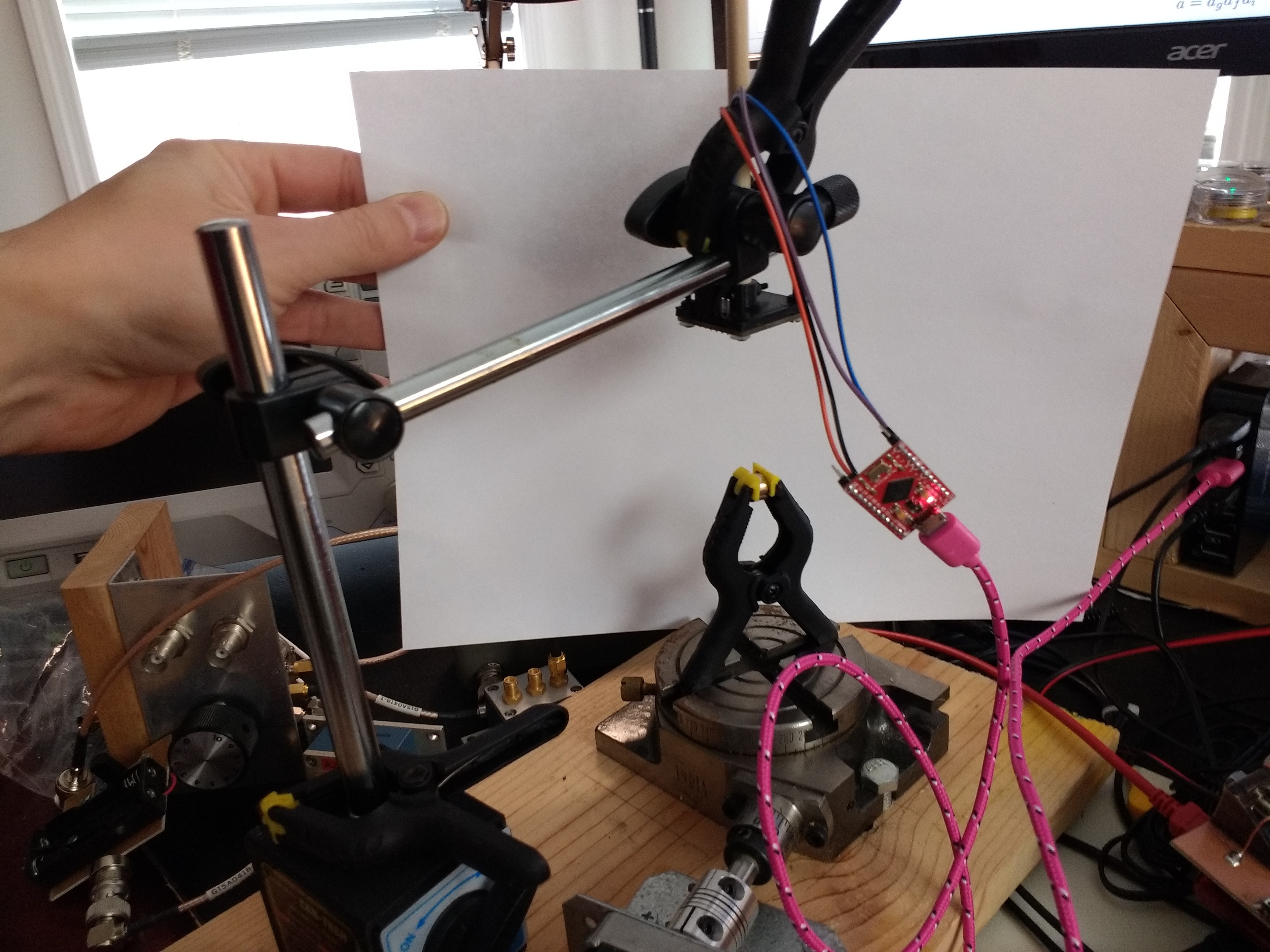
  It's a makeshift goniometer made from a milling machine rotary table.  I had at one point driven the table with a stepper motor, which is still connected, but today I just moved it manually.  A small neodymium magnet is held in the clamp jammed in the table slots.  A MLX90393 eval board is held fixed about 60mm away from the magnet.

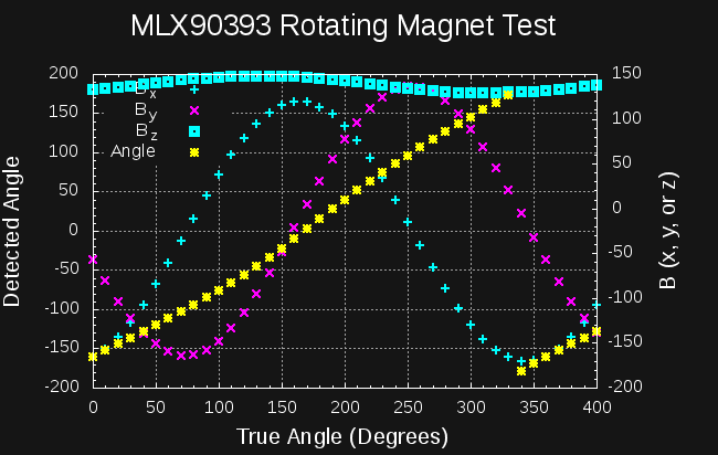
  I recorded data for angles from 0-400 degrees, and made the following plot:

  The x- and y-components of the field show a familiar sine/cosine relationship, while there is just a little variation in z.  This is because the quick setup is not very well aligned.  The resulting angle (determined from 180*atan2(y, x)/pi seems OK,  and is probably usable for many purposes as is.

  The true angle and detected angle have an offset of around 160 degrees because I didn't try to align "0" on the rotary table with the sensor axes at all.
  

  One of the problems is that at this distance from the magnet, the field is close to the same magnitude as the geomagnetic field.  Here's a snippet of the actual data (angle, Bx, By, Bz, T):
  

  0 -165.30 -57.15 132.37 19.96
  10 -156.60 -80.70 133.83 20.09
  20 -143.85 -103.35 134.79 20.09
  30 -127.35 -122.85 136.97 20.13
  40 -107.55 -139.20 138.42 20.09
  50 -84.75 -151.05 139.63 19.87
  60 -61.35 -159.75 141.33 19.91
  70 -36.30 -163.95 143.26 20.18
  80 -11.25 -162.90 144.47 20.11
  90 14.55 -157.80 145.68 20.20
  100 37.95 -148.05 146.65 20.33
  110 59.70 -133.50 147.14 19.98
  120 79.05 -116.55 147.62 20.22
  

  For more accuracy, you could calibrate the system, but this would change if you re-oriented the setup in space, since the geomagnetic field would change relative to the sensor.  Instead, it might be easier to move the magnet closer, increasing the field and diminishing the influence of the big magnet we live on.

  There's probably something fancy you can do to incorporate the z-axis data, too, but I can't think of it at the moment.  I bet there are some compass calibration algorithms that could clean this up a bit.
  

• MLX90393 Datasheet Revised

  Ted Yapo • 01/11/2018 at 19:18 • 1 comment

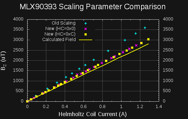
  There has been some activity over on GitHub about the MLX90393 Arduino driver, and it caused me to take another look at the datasheet.  Guess what?  They changed it!  The scaling parameters are different now, which makes the output more accurate.  I had to revive my Helmholtz coil to test it.

  The new scaling factors and a previously undocumented HALL_CONF field (hall effect configuration?) field, which selects 2- or 4-phase hall plate spinning, are in the code and being tested.  After a bit more mileage, I'll merge them into master.  So far, the results are encouraging:

  You can see the scaling numbers in the new datasheet are much closer to the calculated magnetic field in the Helmholtz coil (about 10% high).  I previously measured the coil against the Earth's field and estimated it to be within 2%, so there's room for improvement, but it's getting closer!

  The temperature compensation for the part is still mysterious and doesn't seem to work for me.  I'll have to dig into the new version of the datasheet a little more closely to look for clues.
  
  

  Temperature compensation appears to be working, as long as you remember to set the offsets relative to 0x8000.
  

  At one point, I figured out how to get accurate offset values using a modified compass calibration algorithm.  I'll have to revisit and publish it.
  

• MLX90393 Breakouts Commercially Available

  Ted Yapo • 02/18/2017 at 21:04 • 0 comments

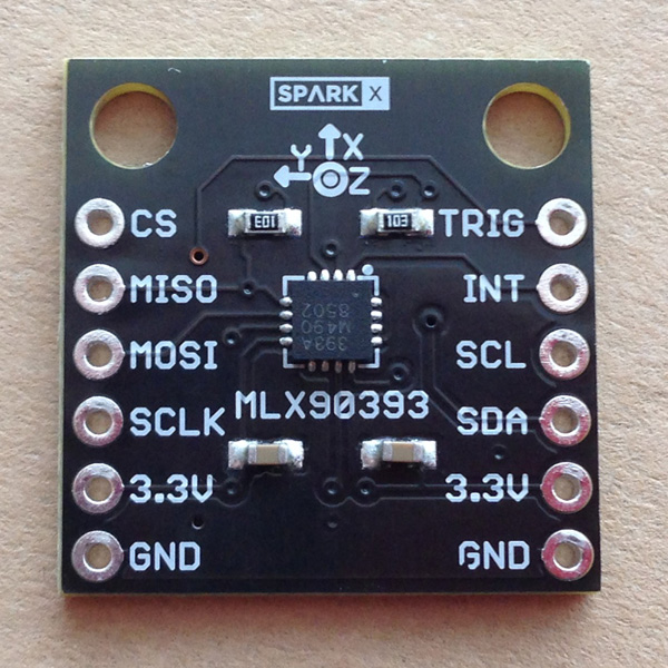
  Sparkfun has made an MLX90393 breakout board the first in their new SparkX series of products, as mentioned recently on the Hackaday blog. I'm not going to make this log an advertisement for them, but if you wanted to get started with this sensor, this is a reasonable way to do it.

  (image linked from SparkFun's site - click here for their product offering)

  I haven't used one of these breakouts personally, but they seem to have the basics covered. There's no mention if the board contains nickel (ENIG finish) or if the capacitors are special non-magnetic types (I can pick up Adafruit's HMC5883L breakout with a magnet due to the ferrous terminals on their SMD capacitors! - but that probably doesn't matter if you use it as a compass and perform hard iron calibrations). If you are using these things inside variable magnetic fields (especially over very wide dynamic ranges), any ferromagnetic material like that can cause problems as it becomes slightly magnetized in the strong regions of the field, then is mis-calibrated in subsequent weak regions. But, even if it has nickel on the board and iron in the capacitors, it should work well enough for almost all practical uses.

  Anyway, Sparkfun said nice things about this project and my driver code, so they must know what they're doing :-)

• Scramble Winding: Take Two

  Ted Yapo • 07/28/2016 at 18:01 • 0 comments

  @peter jansen had an interesting take on my earlier Monte Carlo simulations exploring the effects of scramble-winding coils vs neatly layered windings. He wondered how the angle of the field was perturbed by the random windings - my previous simulations had all examined just the magnitude of a single component of the field (in the axial direction). It turns out that the framework I'd put together for the earlier analysis just needed a little tweaking to examine angles.

  Here's a representation of the field vectors at each point, Pk, in space:

  Br is the field vector in the center of the reference coil - in this case, a 40mm radius Helmholtz coil with two single-loop windings, while Bf is the field vector for a particular sample of scramble-wound coil. The angle between the fields can be calculated by:

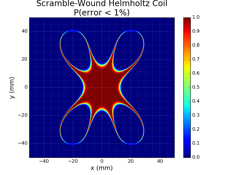
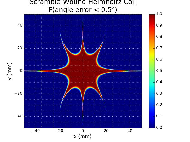
  I already had the code to draw contour areas based on thresholding scalar values, so I substituted this angle for the previous magnitude criterion. As before I ran 10,000 randomized simulations of scramble-wound coils, then used symmetry for an equivalent 40,000 samples. I'll skip presenting the individual images here, and jump right to the probability distributions:

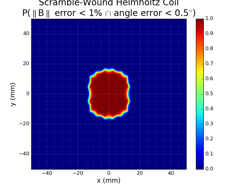
  The left image is the magnitude distribution from before: the colors indicate the probability of achieving less than 1% error in the x-axis component of the field. On the right, we see the new analysis: the probability that the angle of the generated field vector is within 0.5 degrees of the reference field direction (equivalent to a 1-degree wide cone around the reference). Note that the reference here is the field in the center of the reference coil; not the field at the the corresponding spatial point in the reference field. The shapes of the level curves look complementary or "dual" in some vague but satisfying way.

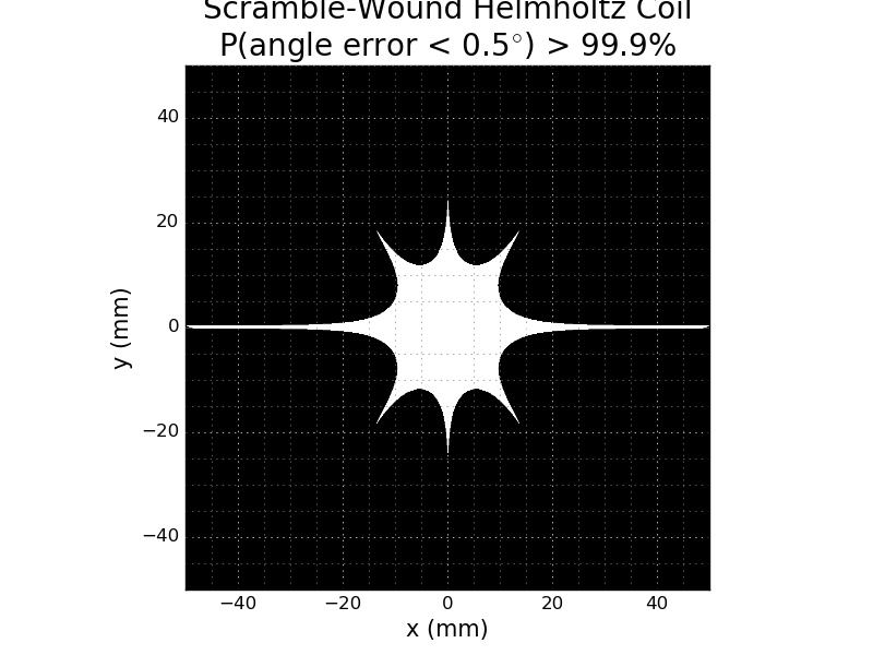
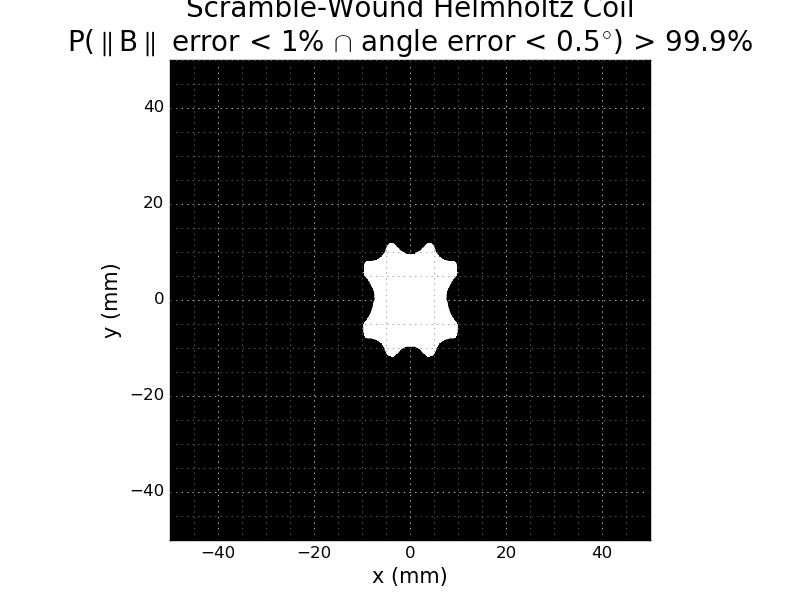
  Like the magnitude version, the angle plot is difficult to read; to get a better view, I again thresholded the probability. This plot represents the area in which you have a 99.9% chance of the field being within 0.5 degrees of the reference (I have to figure out why the title text is getting cut off):

  Of course, you might care about both magnitude and direction. Here's a similar pair of plots for the logical and of the conditions: P(magnitude error < 1% and angle error < 0.5 degrees):

  In this plot, I've used the total magnitude of the B field, instead of just the x-component magnitude as in the others. The right image is again thresholded at 99.9%. The thresholded region encloses a sphere of 15mm diameter, just a little smaller than the 16mm using the magnitude criterion alone.
  

  I'm planning to add a version of this code to the GitHub repository, but I have to clean it up a bit, and make a decent API for the two pieces. Another thing to add to the to-do list :-)
  

• Arduino MLX90393 Library

  Ted Yapo • 07/23/2016 at 22:19 • 2 comments

  I'm probably not going to use an arduino as the controller for this project, but I realize a lot of people do use them, so I wrote what I think is a pretty comprehensive arduino library for interfacing with the MLX90393 over I2C. The code is here on GitHub. If you use it with a 5V arduino board, remember to include level translators to avoid damaging the MLX90393, which doesn't have 5V-tolerant I/Os. You have the option of connecting the DRDY line to one of the arduino inputs for the end-of-conversion signal or using a timed-conversion mode based on the timings in the datasheet.

  So far the code has just a little mileage on it, so watch for anything funny. The basic functions all seem to work.

  After having to deal with the way the arduino build system handles includes, I feel like I need a shower. Ick.
  

• Scramble vs Layered Winding

  Ted Yapo • 07/20/2016 at 16:08 • 2 comments

  I wind a lot of coils. Mostly, they're for RF use and either on toroids, or just simple free-standing air-core coils. I'm always careful to wind them neatly. When I started winding coils for testing magnetometers, however, I found I couldn't easily wind neat, layered coils on these particular spools by hand. @peter jansen solved this problem by building a nice coil winder. Being the impatient type, I took the other approach - scramble winding (aka jumble winding). We've all seen this done on on electric motors and other "electromagnet" components, and I even remember seeing some RF chokes from the vacuum tube era wound like this. What does this type of "random" winding do to the magnetic field? I decided to run some Monte Carlo simulations to find out.

  Unfortunately, the tool I had at my disposal, the python loopfield package I wrote earlier, was painfully slow - each simulated coil took about two minutes to run on my laptop. If you've looked at the code, you know the dirty little secret - the first version was not vectorized. An evening of coding, and the newest version (on github and pipy) is vectorized over the field points, greatly speeding execution. Simulations on my laptop went from two minutes to about 1.6 seconds each (and a decent portion of that is for writing output images) - much better for doing thousands of Monte Carlo runs.

  While I remember - the bug in matplotlib I stumbled into with the field-line plotting is known, fixed, and closed and will be rolled into the next point release. For now, the linked bug report has a better patch than my earlier suggestion.

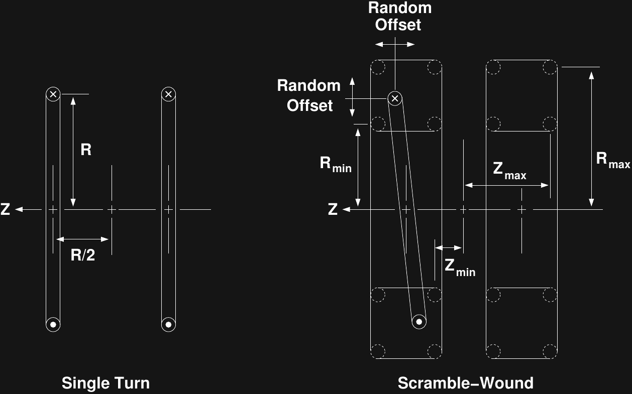
  Here's the model I used for scramble-wound coils. If you can think of a better one, let me know. I tried to capture the constraints that go into an actual coil:

  The 100 turns are still organized into 10 rough "layers" - each of the 10 turns within a layer is assigned a nominal radius, then this value is perturbed by a uniform random floating point value between -5 and 5 winding spacings (the coil form is 10 "spacings" high). The idea is to capture the fact that turns may not have a well-defined radius, but constraints of winding the coil onto the spool still enforce an approximate layering. Similarly, in the axial direction, the turn position within the winding is perturbed uniformly between -5 and 5 row widths. These perturbations allow a loop nominally in the exact center of the winding to end up anywhere within the coil form. Since the coil really is in 3D, the off-axis tilt is moved into a random radial direction instead of remaining in the plane as the diagram might suggest. The center position (which may now be off the central axis) and the loop normal (which is generally no longer in the z-direction) are calculated from the nominal coil locations and offsets. This model assumes infinitely thin current loops, so there's no allowance for minimum spacing between windings - it's possible the model could place loops in exactly the same space (certainly closer than finite-diameter wire would allow). This perhaps isn't the best physical model for scramble-wound coils, but I think it's on the conservative/pessimistic side, and should at least give a qualitative feel for how the field uniformity is affected by "random" windings.

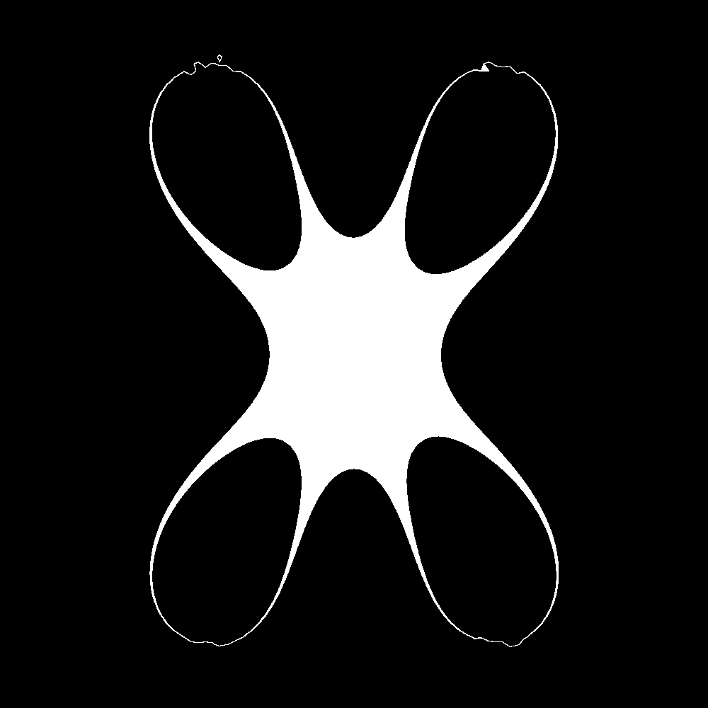
  I ran 10,000 simulations of coils randomly generated in this way (using the numpy.random.random_sample() function, which I believe uses Mersenne Twister underneath). To analyze the results, I plotted the 1%-error contour area (relative to the two-loop reference coil) to a series of PNG images. Here are some representative images generated by the random sampler (the left image has the smallest area of the 10,000 samples, the right image has the largest, and the middle was arbitrarily chosen):

  I think the left-most image is a pathological case; my simple model for random coils can easily generate non-physical arrangements of windings. Until I come up with a better model, I'll have to rely on a statistical approach.
  

  I wrote a second...

  Read more »

• Duh! and Scans!

  Ted Yapo • 07/10/2016 at 14:39 • 2 comments

  Offset Calibration (Duh!)

  Sometimes it takes me a while to "get it." Unfortunately, in this format "a while" may be several build logs. This is one of those cases. The original sensor I was using, the HMC5883L, is intended as a compass sensor. Calibration of compass sensors is a well-studied problem, and information about how it works and how to perform it abounds. I had initially dismissed using a compass calibration procedure for the scanner since it only calibrates ratiometric accuracy (the relative scaling of the x-, y-, and z-axes) - exactly what you need for a compass, but not terribly useful for absolute field measurements. In the usual procedure, a large number of measurements are taken with the sensor in random orientations in the geomagnetic field. Plotted in 3-space, the measured field vectors lie on an off-center ellipsoid. Calculating the transformation required to make it a sphere gives you the relative sensitivities of the three axis sensors, while centering the sphere yields the offset. Exactly the offset I need to program the MLX90393 temperature compensation. I think combining a modified "compass calibration" for offsets with some field-coil measurements for scale calibrations will probably work. I'll be exploring this, and will post the results once I have something usable.

  Scans!

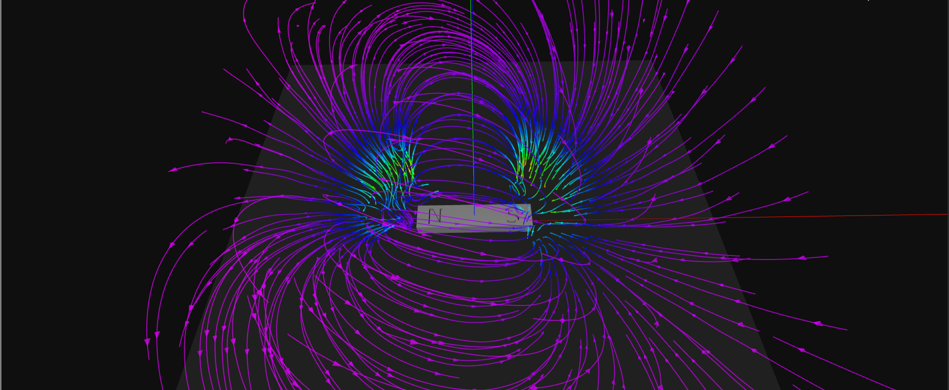
  I got the original demo code re-factored to the point that I can make new scans now. I also wrote field-line integration code in JavaScript so it can run live in a browser, and performance really isn't too bad. For now, I'm using simple Euler integration, but I found this paper on particle tracing in vector fields which explains a higher-order Runge-Kutta method which I will implement going forward. Then there's the topic of interpolation method; for now, I'm just using a simple trilinear interpolation, but I'm going to look into other methods to see if they can provide more accurate results. In any case, here's a low-resolution test scan of a small permanent magnet, captured with only 7x13x13 samples:

  This visualization was done with no calibration whatsoever - no baseline scan, and no offset or scaling from the raw MLX90393 data. It's not numerically accurate, but qualitatively it looks like I'd expect - field lines in loops from north to south. I made a quick model of the magnet in OpenSCAD - this kind of model will be useful when scanning around items: the path-planning code can use such models to avoid collisions with the scanning probe. You can see me sneaking in to measure the magnet during this video of the scan. Remember, don't put your hands inside the printer while it's running. The video is sped up - for now, the scanning is very slow, taking about 20 minutes for this scan, but I think this can be improved quite a bit.

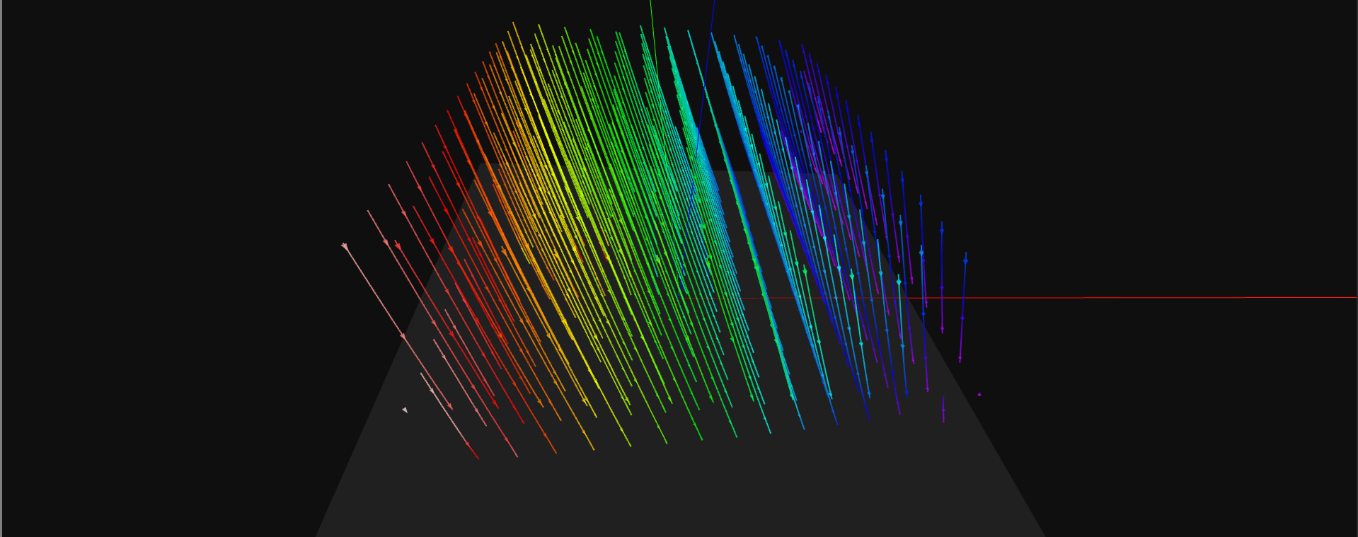
  Watching the scan is a little like watching grass grow. I wanted to show it, however, to illustrate the type of magnetic "clutter" one typically finds in a 3D printer: stepper motors and steel rods and frame. How much does that affect the scan? I'm starting to find out. Here's an identical baseline scan taken with the magnet removed:

  The colors aren't on the same scale between the two plots; the code currently stretches for maximum dynamic range. The baseline, which should consist just of sensor offset and the geomagnetic field, has a range of 141-228 μT, while the bar magnet shows a range of 13-11,485 μT. The interesting thing about the baseline scan is that the field appears to be fairly uniform, except for a slightly stronger field on the negative-x (left) side of the volume. Is that the influence of the stepper motor on the upper left of the video? I'm not sure yet. What appears to be the case is that this baseline is repeatable - I've seen similar fields with each "empty" scan. I haven't diff'ed baseline scans yet to get a quantitative comparison, but so far, it looks like you could correct for this quite easily. The code isn't quite where it needs to be to apply such a correction, but that's...

  Read more »

• MLX90393 Temperature Compensation Tests

  Ted Yapo • 07/08/2016 at 17:14 • 1 comment

  After some discussion with the application engineer at DigiKey and a bit of hacking, I think I understand how temperature compensation on the MLX90393 works well enough to incorporate it into the driver. It will take some time to re-write the code incorporating what I've learned, but I wanted to get this documented while it's still fresh. I might be wrong about any or all of this; if you notice an error, or have different information about this part, please let me know. Part of the problem is that the factory-supplied parameters just seem to give lousy results, so for a long time I figured I was using the part incorrectly. I don't think so anymore.
  

  Temperature Sweeps on the Cheap

  To test temperature compensation, you need to have a way to sweep temperature. I actually have a cobbled-together environmental chamber consisting of a thermoelectric heater/cooler controlled with a decent thermostat. However, using it for these experiments was inconvenient, so I used a simpler technique. Since the MLX90393 has an on-die temperature sensor, you can generate temperature sweeps by heating (or cooling) the part and collecting data while it drifts back to ambient. This technique has a few potential problems, including the accuracy of the on-die temperature sensor and the exponential temperature curve. The later causes the temperature to move too quickly at the beginning (hot or cold) of a sweep, and too slowly as the part equilibrates to ambient. You might improve the technique with an insulating blanket (say of Styrofoam) slipped over the part after the initial heating/cooling, then removed once the sweep rate drops. I didn't bother.

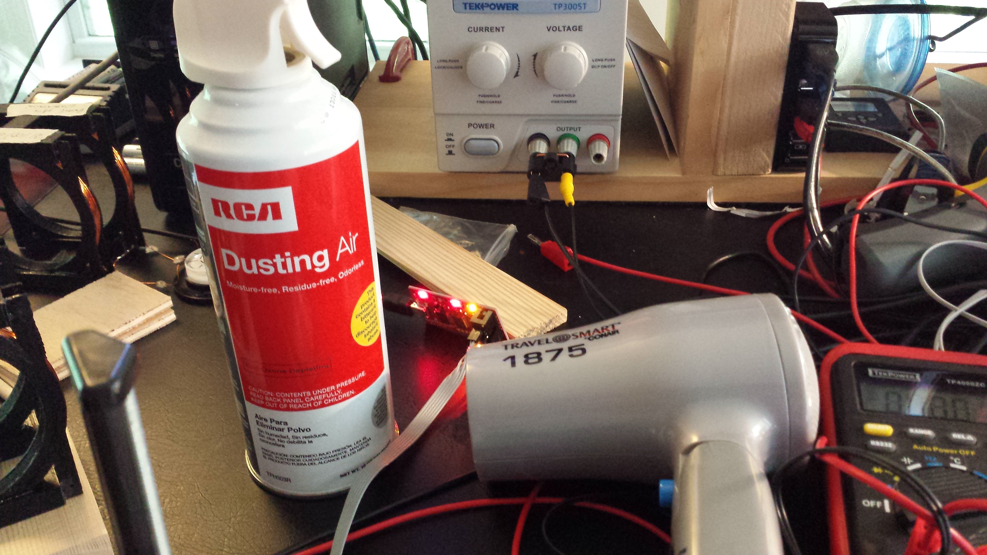
  Here are the tools of the trade:

  The "canned air" is actually 1.1-Difluoroethane, a refrigerant with a boiling point of -25C. The label explicitly tells you NOT to spray with the can upside down, so don't do it! But when you do, you get a stream of liquid coolant instead of the gas. A brief shot of liquid on the device-under-test brings it below 0C to start the cold sweep. This is much cheaper (and more widely available) than official "cooling spray." The hair dryer (which I could use in my youth, but is unnecessary now) is self-explanatory. I didn't use a heat gun since it would be too easy to harm the PLA printed components, epoxy, or even solder joints. Here's a plot of a typical temperature profile for the part mounted in my epoxy potting:

  The datasheet lists -20 to 85C as the operating temperature range, but I'm going to assume people can make do with a more narrow range in the magnetic field scanner.
  

  Configuring Temperature Compensation

  As far as I can glean from the available documentation, the on-chip temperature compensation algorithm is controlled by 7 parameters:

  • TCMP_EN : boolean which enables temperature compensation
  • TREF : breakpoint for piecewise-linear compensation algorithm. Factory trimmed
  • Sens_TC_HT : high-temperature compensation coefficient. Factory trimmed
  • Sens_TC_LT : low-temperature compensation coefficient. Factory trimmed
  • Offsets (x, y, z) : "offsets" for x, y, and z

  TCMP_EN is self-explanatory, and TREF and the two coefficients are programmed into nvram at the factory (more about this later...), leaving just the offsets to figure out. The datasheet is not exactly lucid about the offset parameters:

  OFFSET_i[15:0] : Constant offset correction, independent for i = X, Y, Z

  Probably realizing this, Melexis was kind enough to write a simplified "getting started" document explaining how to use this part. Here's the section concerning the offset parameters:
  

  OFFSET_X, OFFSET_Y & OFFSET_Z
  These parameters are used to compensate the offset in case the temperature compensation is enabled. They are not used with TCMP disabled. Please refer to the application note on the temperature compensation for more info. These values can be blindly programmed to the values given in this document (if not already programmed).

  The values come programmed to zero in the nvram, and no values are actually given...

  Read more »

• 3-Axis Coil Design and Interesting Tangents

  Ted Yapo • 07/07/2016 at 00:12 • 7 comments

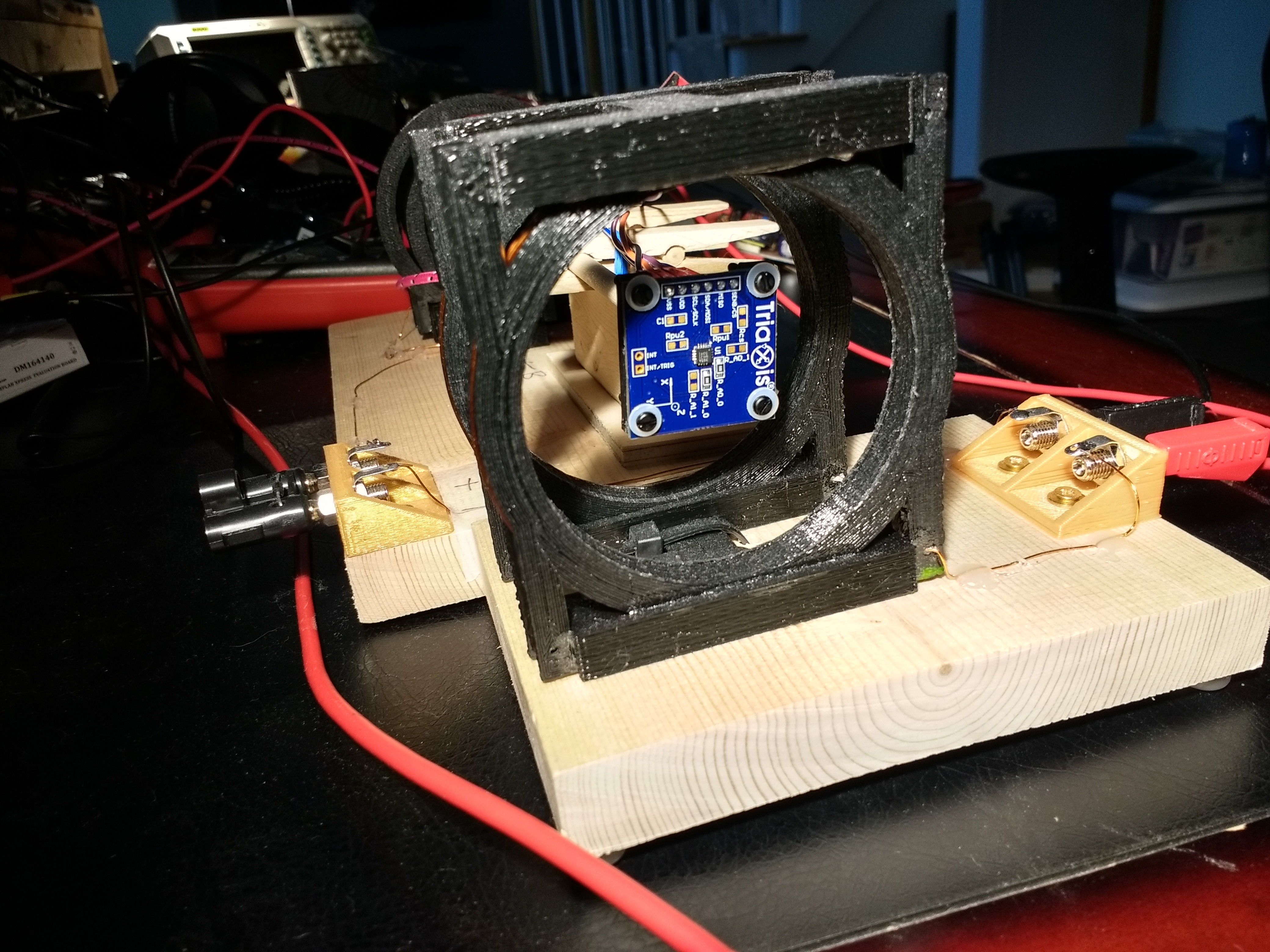
  I got temporarily obsessed with designing a 3-axis field coil to calibrate the MLX90393 sensor. A 3-axis coil would allow all three axes to be calibrated with the sensor in a single position. This allows for easy detection and compensation of angular errors: not aligning the sensor exactly with the coil axes. In addition, a 3-axis coil would make it easy to register the magnetic coordinate system of the sensor into the spatial coordinate system of the printer - this is sure to be slightly different each time you mount/detach the sensor head.

  I started playing with 3-axis Helmholtz designs, but for multi-turn windings, the required spacing makes for a clunky design. Here's one of the mock-ups I was playing with:

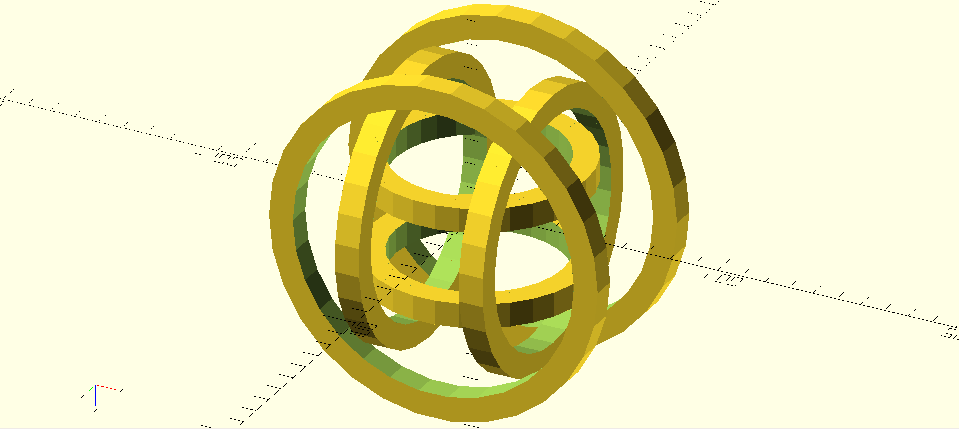
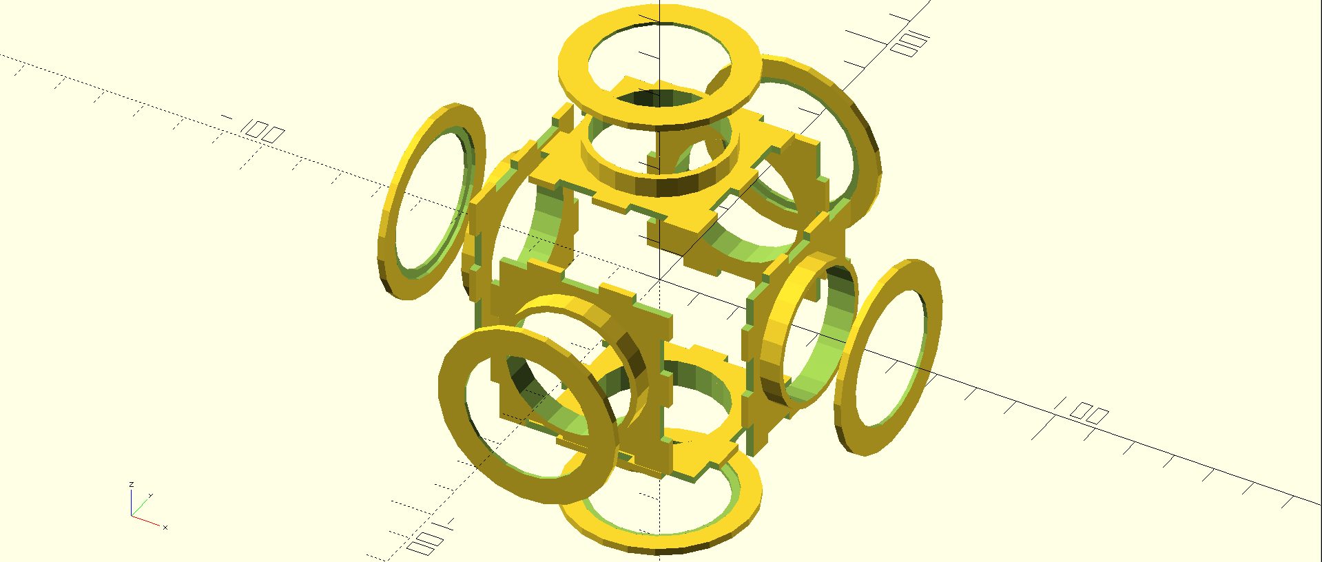
  The size of the windings also allows only a very small active volume, and the nested configuration complicates the mechanical design (which I didn't complete). I started to wonder how important the spacing was in the Helmholtz design. If the spacing constraints could be relaxed, I could use something like this:

  Here, the windings are farther apart than in the Helmholtz design. This allows the windings to be on the cube faces, which are all the same shape, and all the parts can be conveniently printed "flat" on the printer bed. I printed a few of these, and they're fun to snap together (the spool caps have to be glued). Mechanically, this is a win, but I had no idea what this does to the field, so some simulations were in order.

  Unfortunately, the math I'd done so far could only calculate the field along the coil axis; the field in the full volume of the coil was unknown. I downloaded some finite-element software ( Elmer, a general-purpose package, and MaxFEM, aimed solely at magnetics) and played around a bit. These are powerful tools with steep learning curves, and while I'm going to keep at it and learn to use them eventually, using them for my immediate needs feels like slicing bread with a chainsaw. So, I decided to write the "bread knife" of field coil design.

  I lucked out and found the paper Simple Analytic Expressions for the Magnetic Field of a Circular Current Loop on the NASA Technical Reports server. This paper provides equations for the full vector field surrounding a loop of current, and the equations are fairly simple, in part because the required elliptic integrals are conveniently hidden. To my great joy, I found that the python scipy package contains routines for numerical evaluation of these integrals, greatly simplifying field calculation. Since the field obeys superposition, these equations can be used to calculate the field surrounding any 3D configuration of circular current loops - which covers just about any coil I might think of using. I was able to create the core of a python simulation fairly quickly; it's less than 100 lines of code. Having the simulation as a library is very convenient - you can program all sorts of analyses and what-if's easily.

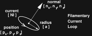
  Here's the model for the "filamentary" current loops simulated:

  The loop is assumed to be a conductor of infinitesimal diameter, centered in 3-space at position p, of radius a, with normal n, and carrying a magnetizing current NI. For normal "magnet wire" in relatively large loops, this model will work very well.
  

  The "loopfield" code is here on GitHub, as well as on PiPY ('pip install loopfield' gets you a copy, but check out the examples on GitHub). It requires matplotlib for the plotting functions, but the core engine just uses numpy and scipy. Usage is very easy - here's code to calculate the vector field for a single-turn coil:

  #!/usr/bin/env python3
  import loopfield as lf
  # create empty field with specified units
  field = lf.Field(length_units = lf.cm,
                   current_units = lf.A,
                   field_units = lf.uT)
  # single-turn 10 cm x-oriented coil at origin
  position = [0., 0., 0.]
  normal = [1., 0., 0.]
  radius = 10.
  current = 1.
  c = lf.Loop(position, normal, radius, current)
  # add loop to field
  field.addLoop(c);
  # evaluate vector field at origin
  B = field.evaluate([0.,...

  Read more »

• Hand-soldering QFN Packages

  Ted Yapo • 07/01/2016 at 16:35 • 0 comments

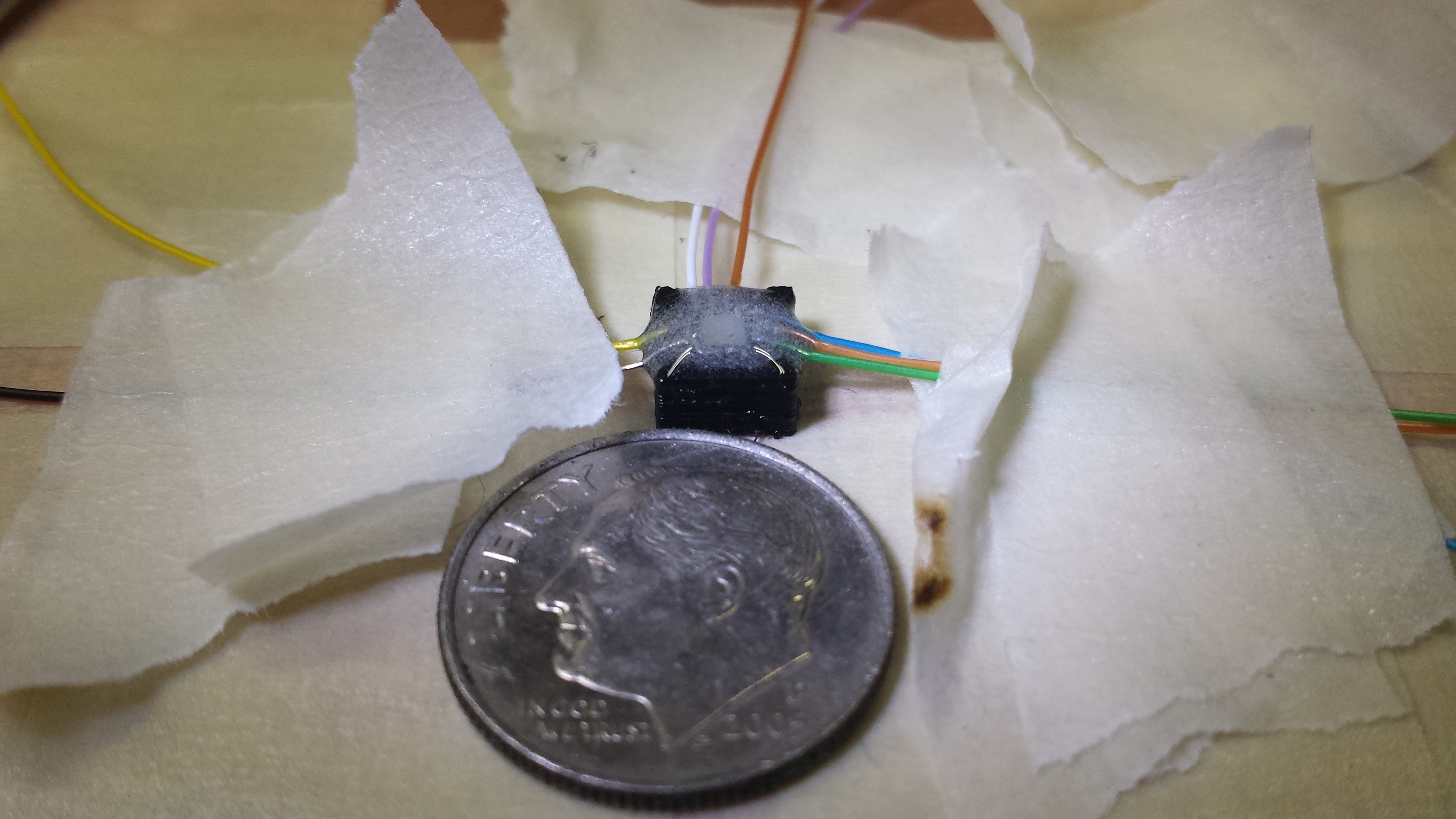
  You occasionally see some questions about whether it's possible to hand-solder SMT parts in QFN packages. This usually refers to mounting them on a PCB. In my case, I didn't feel like waiting for PCBs to come back to start testing the MLX90393 on a smaller scanning head, so I soldered wires directly to the part.

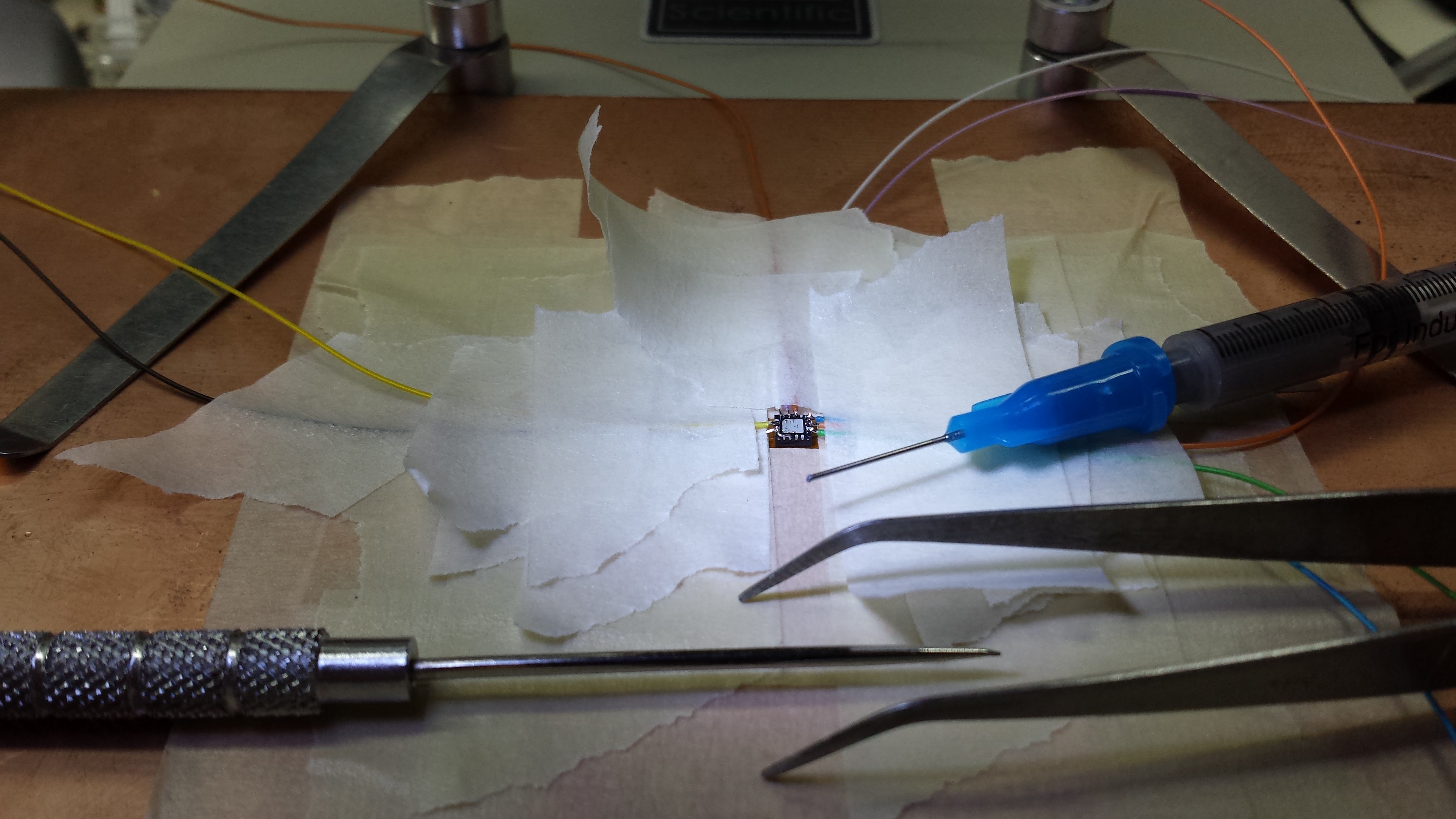
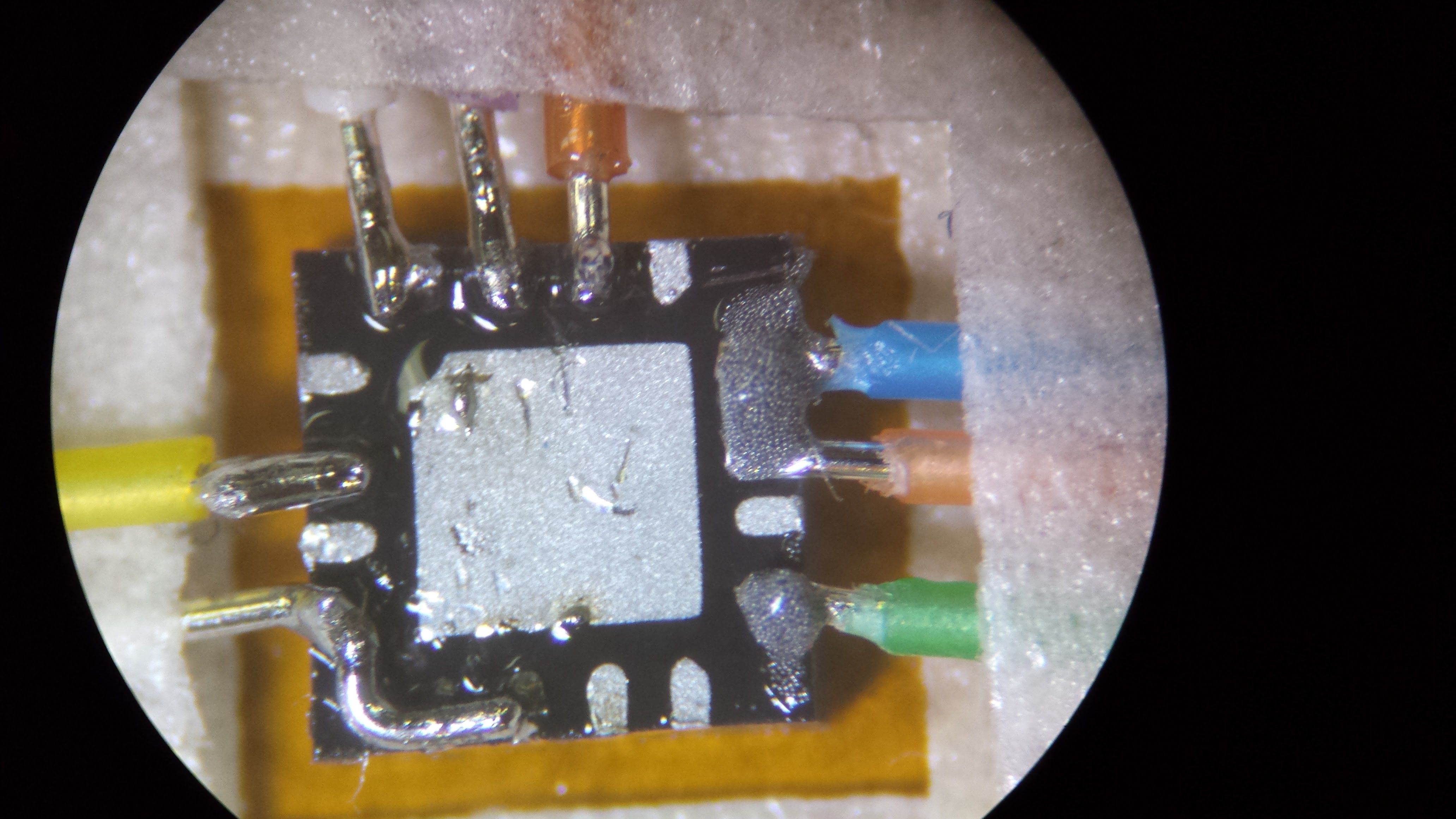
  I held the 3x3mm part down with a piece of upside-down Kapton tape, then used masking tape to hold lengths of 30 gauge kynar-insulated wire-wrap wire on the pads. The wire is almost a perfect fit for the 0.5mm pitch. A pair of tweezers under the 10x (and occasionally 30x) inspection microscope allowed for fine positioning of the wires:

  To solder the wires, I first coated them in a blob of solder paste using a 25-gauge needle on a 1cc syringe, which allows for much finer application than the larger syringes:

  You can see the individual particles of solder in the paste. I then held the (very large) soldering iron tip near the paste until it melted. A gentle tug on each wire with tweezers ensured that it was really connected.

  This is the second part I've done this way. The first assembly was broken twice, the second time proving fatal. The first mishap occurred while stripping the loose ends of the wires after soldering. The stripper produced too much "pull" on the wire, and tore it off the part. For the second version, I stripped both ends of the wires first, printed a small cup from PLA, and potted the part and wires in epoxy:

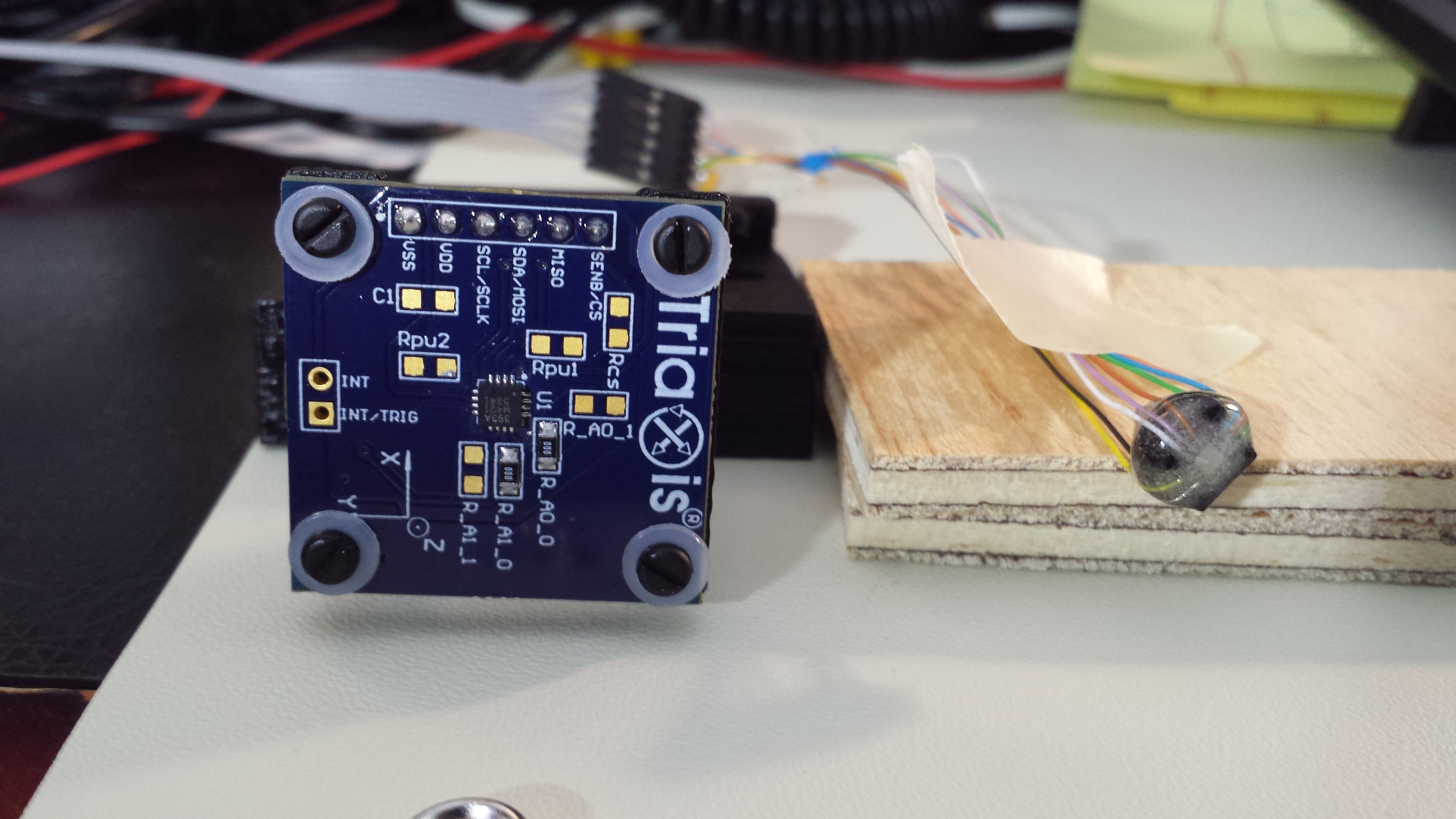
  Here's the completed probe after a second glop of epoxy along side the over-sized evaluation board:

  Much better. And, it works! It's delivering field measurements to my python code as I write this. I'll be more careful with this one. The first attempt worked for a few minutes until I tried to re-align the axes and pulled a wire out of the meager epoxy on that version.

  Making this was a little bit of a pain, but it gives me three things immediately - another sample of the MLX90393 to test, a part not mounted on an ENIG-finish board, and obviously a much smaller probe. It's clearly no substitute for a PCB, but it will allow me to do something now.
  

View all 18 project logs