Bertrand Selva
-
BACKPRESSURE
11/16/2025 at 14:31 • 0 commentsImplementing Backpressure in a No-RAM Pipeline
In the latest version of the project (see attached source), I've introduced a simple backpressure mechanism to ensure that each produced data word is truly consumed before a new one is accepted. Here’s how it works:
The design is 100% synchronous. There is no external RAM, no FIFO. The objectives are twofold:
– Never overwrite an output that hasn’t yet been read.
– Never accept a new input until the previous output is consumed.
For debugging and visualization, the 16 output bits will be connected to a parallel bus, monitored by the logic analyzer.Validation Protocol
The pipeline uses two standard handshake signals:
out_valid: signals that output data is ready.
out_ready: external pulse signaling the data has been consumed.
Control logic is built around:
wire hold_pipeline = (out_valid && !out_ready);
wire step_en = !hold_pipeline;
Pipeline steps forward only if the previous output has been read (out_ready=1). Otherwise, the pipeline is frozen everywhere. Thestep_ensignal then drives all internal enables.
This logic ensures:
– No new input if previous output isn’t consumed.
– No risk of internal overflow, even with zero FIFO.
– The pipeline remains frozen as long as downstream isn’t ready.
That’s exactly what’s needed for streaming scenarios controlled by a slow peripheral or manual inspection.
Signal LegendSignal Direction Role/Meaning in_valid Input External → FPGA: “Input data is present on in_byte” in_ready Output FPGA → External: “I can accept a new input now” in_byte Input External → FPGA: Data to process (8 bits) out_word Output FPGA → External: Output word produced (16 bits) out_valid Output FPGA → External: “Output data is ready, read me!” out_ready Input External → FPGA: “The output data has just been read/consumed” Typical Timing
cycle in_valid in_ready out_word out_valid out_ready Description 0 0 1 -- 0 1 Idle state. FPGA does nothing—no input pending, no output produced. in_ready=1: ready to accept.out_valid=0: nothing to read. The outside can inject a value at any time.1 1 1 X1 1 0 Input received. External presents value on in_bytewithin_valid=1(pipeline ready). The pipeline captures input, computes, produces X1, setsout_valid=1.out_ready=0: output not yet consumed.2 0 0 X1 1 0 Waiting for consumption. Input transfer done ( in_valid=0), output not yet read (out_ready=0). Pipeline blocks:in_ready=0,out_valid=1, output is held stable. Registers frozen, no updates.3 0 0 X1 1 1 Output read. External acknowledges output by asserting out_ready=1for one cycle. The pipeline sees the "green light": data is consumed. X1 is readed by ESP32. On next clock, pipeline will advance and be ready for new input.0 0 1 X1 0 1 Return to idle. After data consumption, pipeline returns to idle: in_ready=1, ready to accept a new word. Cycle repeats as above for the next input.1 1 1 X2 1 0 New input accepted. External detects in_ready=1and injects a new value within_valid=1. The pipeline captures this new input, computes X2, and outputs it. Sequence is analogous to step 1.Key Principles
-
Computation (internal register update) happens only on a clock edge where
step_en=1, i.e.:step_en = !hold_pipeline = !(out_valid && !out_ready)
-
If the output is not consum
hold_pipeline and step_en depending on the statesed (
out_ready=0), the entire pipeline is frozen: no new input, no state evolution, everything held stable. -
in_ready=1only when the pipeline can accept a new input (never if the previous output remains unconsumed). -
The external system dictates the pace: as long as
out_readyisn't asserted, there is no risk of data loss or overflow, as the pipeline remains frozen. The external master sets the tempo.
hold_pipeline and step_en depending on the states
In the idle state, the pipeline keeps stepping on every clock edge, because
step_en = 1as long asout_valid = 0.
Butin_fire = in_valid && in_readystays at 0, since the MCU has not yet assertedin_validto signal that an input sample is available.
Result: the pipeline advances, but always falls into the flush branch of the registers (all validity flags reset to 0, no useful data propagates).In the input-received state, we detect the first clock tick where
in_fire = 1, meaning the input sample is actually being consumed.
On that clock edge:-
the pipeline captures the sample,
-
computes the response,
-
places X1 on
out_word, -
forces
out_valid = 1(data ready), -
while
out_ready = 0(MCU has not read it yet).
The combinational logic then driveshold_pipelinehigh.
On the next clock edge, sincestep_en = !hold_pipeline = 0, the entire pipeline is frozen: no internal register advances as long as the output has not been consumed.The MCU may take as many cycles as needed to read the output and indicate it by asserting
out_ready = 1.
At that moment,hold_pipelinedrops to 0,step_enreturns to 1, and we fall back to the idle state:-
in_ready = 1(ready for the next sample), -
waiting for the MCU to assert
in_valid = 1to indicate new input data.
Then the cycle repeats, sample after sample.
Debug and Visualization
With the 16-bit parallel output, I can easily connect a logic analyzer and verify:
- Each
out_validis matched by a subsequentout_ready - No double writes
- No missing data
Why This Approach?
This architecture is the easier way to do : no RAM, no FIFO. It offers simple, robust control, making it ideal for early prototyping and external capture. While it's not suitable for high-throughput deployment (where a FIFO would be required), this method ensures total reliability in manual or low-rate streaming scenarios. The ESP32 acts as the master: it alternates read and write phases, always transferring a single sample at a time.
-
Computation (internal register update) happens only on a clock edge where
-
USB BLASTER V2 OK
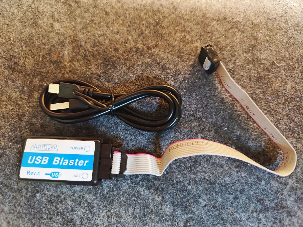
11/15/2025 at 19:27 • 0 commentsI had bought a USB Blaster on AliExpress for 2€.
If it had worked, it would have been great…
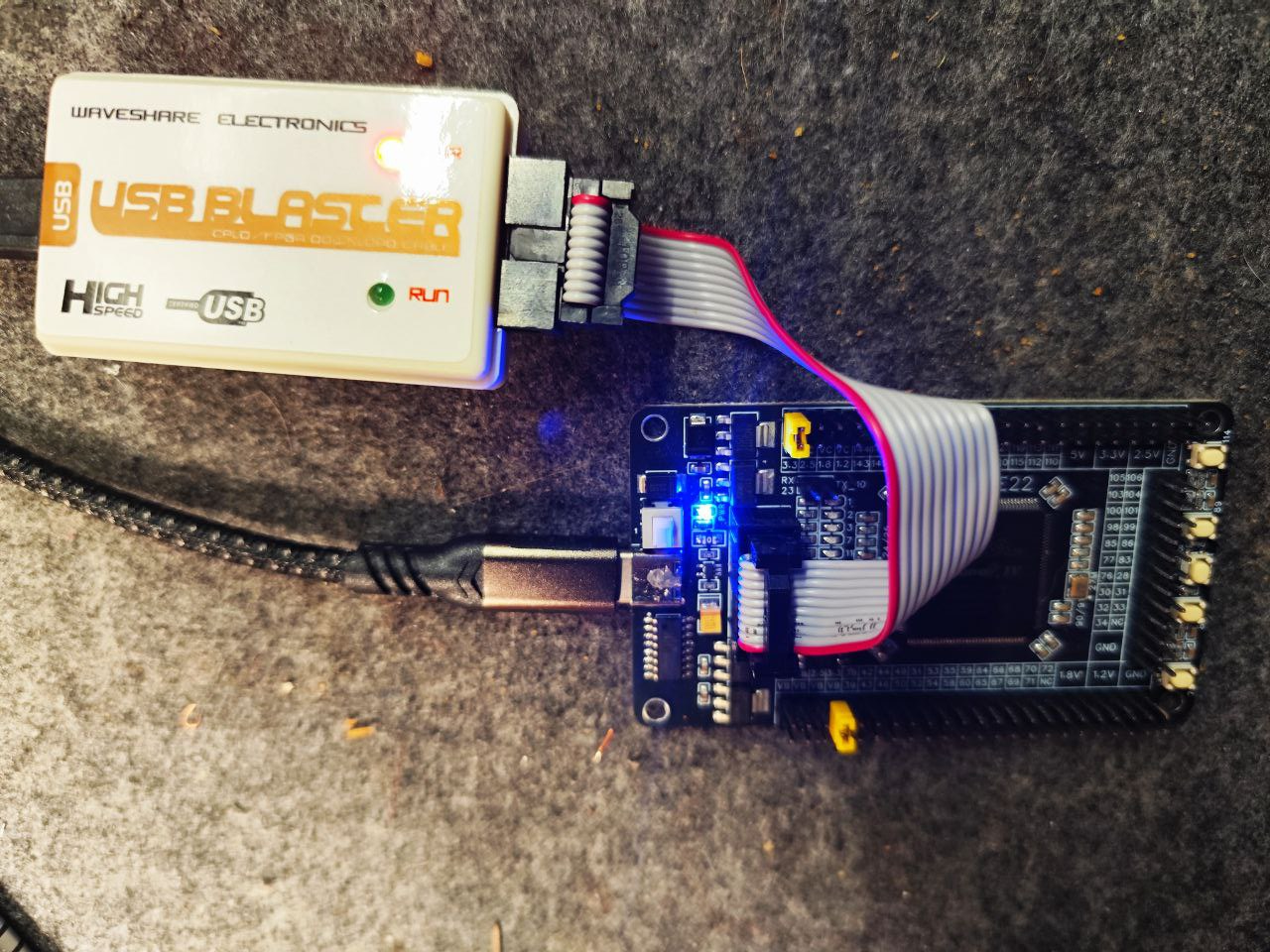
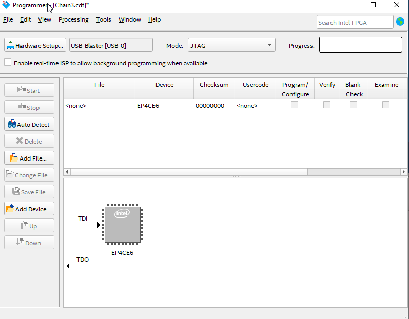
I tried it with Quartus 13 and Quartus 22. Nothing worked: it just wouldn’t function.So I bought a Waveshare Electronics USB Blaster V2, and this time my FPGA was detected immediately and everything worked on the first try with Quartus 22.
I paid around thirty euros for this version, but it actually works perfecty !
The EP4CE6E22 Cyclone IV was detected at the fisrt try....
At the same time, if I’d bought the 10-wire ribbon cable on its own, it would have cost me more than 2€. I don’t have the motivation to open it up and see what’s inside. But it’s definitely better to go for another model…
-
64 TAPS RNS FIR
11/10/2025 at 16:34 • 0 commentsI’ve uploaded the new version of the RNS-based FIR filter, now extended to 64 TAPS (see PROGRAMME16BITS_FIRCOMPLET64TAPS.zip in project files) .
Everything is OK !FIR Coefficients
The implemented coefficients are:
h_int =

Columns 1 through 29
  0   0   0   0   1   1   2   2   3   3   2   1  -1  -3  -6  -9 -11 -13 -14 -13  -9  -4   4  15  27  40  54  68  81

Columns 30 through 58
 91  98 102 102  98  91  81  68  54  40  27  15   4  -4  -9 -13 -14 -13 -11  -9  -6  -3  -1   1   2   3   3   2   2

Columns 59 through 64
  1   1   0   0   0   0
These coefficients come from a windowed sinc with a normalized cutoff frequency of 0.1.
They were scaled so that the sum of all taps equals 1024 (2¹⁰), allowing normalization after CRT reconstruction by a simple 10-bit right shift, with no hardware divider required.
All multiplication LUTs were completely rewritten to match these coefficients. The updated code is available in lut_verilog_64TAPS.v.
Implementation results
Target: Cyclone IV GX EP4CGX22BF14C6
Tool: Quartus Prime 22.1std.2 (Lite Edition)Metric Value Logic elements 16 007 / 21 280 (75 %) Registers 7 982 Embedded multipliers 0 / 80 (0 %) Memory bits 0 / 774 144 (0 %) PLLs 0 / 3 (0 %) Max frequency (Slow 1200 mV 85 °C) 96.9 MHz This confirms that the 64-tap RNS FIR is entirely built from logic elements only, with no DSP usage : a fully LUT-based architecture.
Next step — Now that everything works:
Decouple the input data rate from the FPGA clock so that the 64-tap pipeline can handle inputs slower than clk without any data loss or misalignment, and simulate the full chain to verify correct behavior.
Then move on to the hardware implementation of the FIR.
-
First Functional RNS FIR
11/09/2025 at 17:36 • 0 commentsI continued exploring FIR filtering in RNS on the Cyclone IV, in line with what was presented in the previous log. This log introduces an RNS-based FIR filter that does not rely on the FPGA’s DSP blocks, uses no conventional multipliers, and is implemented entirely with combinational logic and LUTs.
Sizing and Initial Limits
I started with a 128-tap FIR, as defined in the previous log.
In that form, it did not fit in the Cyclone IV E22.![]()
Compilation reported around 30,000 logic elements when not exploiting coefficient symmetry for a 128-tap FIR. By taking advantage of symmetry (which is generally required for linear-phase FIR filters and is a common configuration), the logic usage drops to around 15,000 logic elements for the same filter length. Even if this does not completely saturate the device, this kind of “full logic” architecture quickly eats into the available budget, especially on a family like Cyclone IV.
With a symmetric implementation, it should be possible to push a 128-tap FIR with 16-bit input data and an effective dynamic range of about 2³⁷. That would be very close to the practical upper bound on this FPGA.
Minimal FIR: Validating the Pipeline
Since I had to abandon the initially targeted filter, and in order to simplify debugging and verification, I implemented a symmetric 4-tap FIR with coefficients (1, 3, 3, 1), without exploiting symmetry internally. The goal was to preserve a general architecture that can be reused for non-symmetric filters if needed.
In this configuration:
-
Around 2,800 logic elements are used
-
No embedded RAM, no DSP blocks, no conventional multipliers
Simulation becomes manageable again: each pipeline stage is easier to track, and debugging is more straightforward. This makes it a useful intermediate step before moving back to longer filters. The code is provided in a ZIP file attached to the project files.
The design works. The maximum achievable frequency is about 100 MHz.
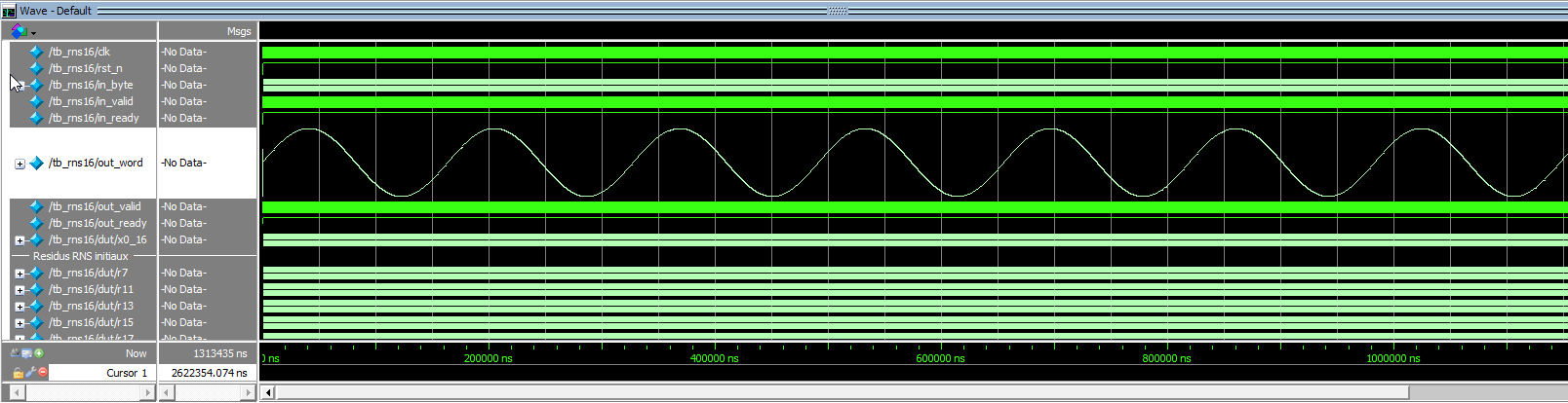
To validate the behavior, I injected a harmonic input over 8,192 samples, covering the full dynamic range.![]()
The filter output matches the expected response, confirming that the FIR operates correctly in RNS, using only pure logic (including the full pipeline: the FIR itself plus the two correction stages).
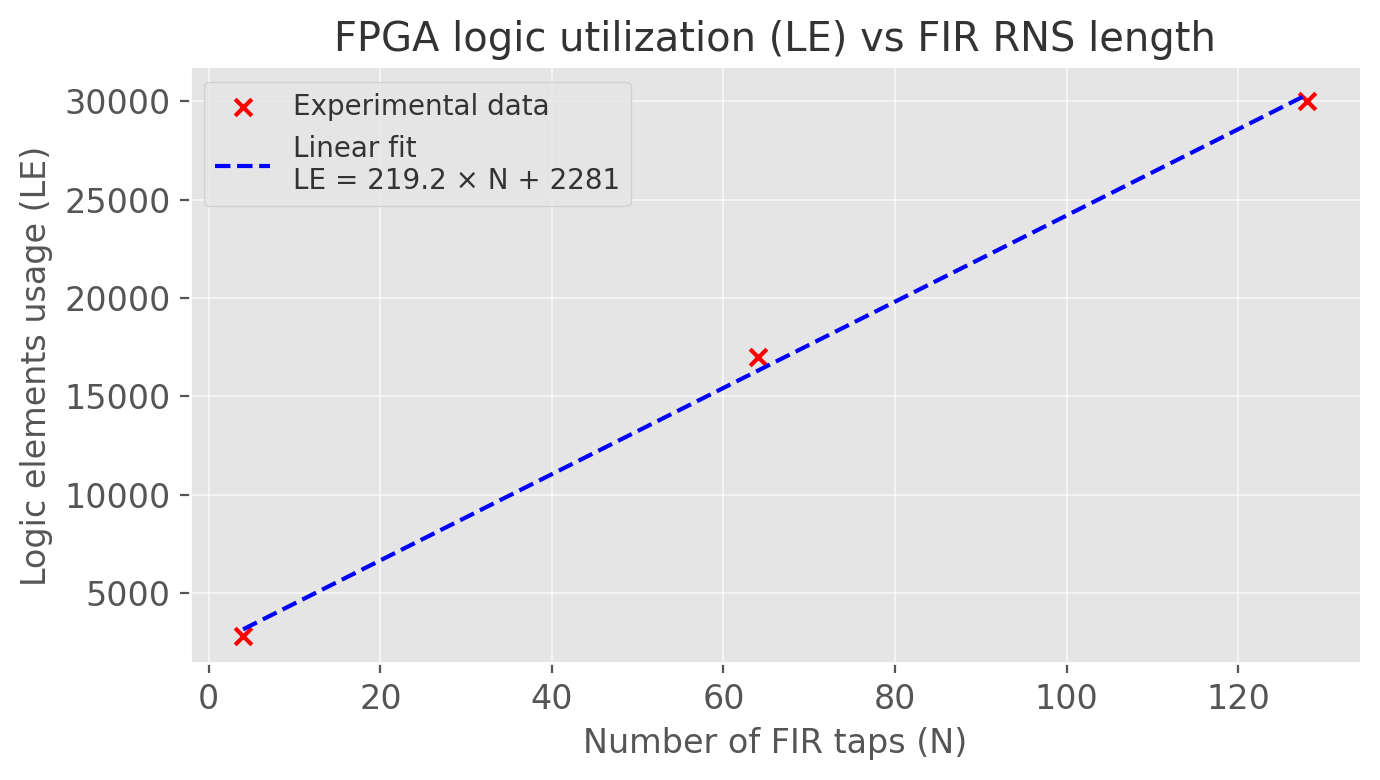
Scaling Law
These results show that it is possible to implement an RNS FIR on a standard FPGA with 0 RAM and 0 DSP usage. The following figure shows the (approximately linear) relationship between FIR length and logic element usage.
![]()
From the measured points, the logic usage scales approximately as:
LE≈220×N+2200
(there is likely room for improvement with a more optimized implementation, but this gives the correct order of magnitude).
For a symmetric FIR, a reasonable target is about:
LE≈110×N
What RNS Really Enables on FPGA
These results help reassess where RNS is relevant in this kind of architecture. RNS is not meant to replace binary arithmetic, but it is a useful tool in the FPGA designer’s toolbox, with clear advantages in specific contexts.
On an FPGA like the Cyclone IV E22
Even with hardware multipliers available, a fully parallel FIR quickly runs into constraints related to accumulation, routing, pipelining, and overall logic usage. The limitation does not come only from the number of multipliers, but also from all the surrounding logic: adders, registers, fan-out, and dataflow control.
For example, the EP4CE22 provides 66 DSP blocks with 18×18 multipliers (suitable for 16-bit inputs). This is enough to parallelize a binary FIR up to about 64 taps; that is roughly the practical upper bound for a fully parallel implementation. Even in that configuration, the logic elements are still used: they are required to build the adder tree that sums all multiplier outputs.
It is noteworthy that, on the EP4CE22, both approaches, binary with DSPs and RNS with pure logic, end up constrained to FIR filters of about 64 taps, even though the resource distribution is very different:
RNS uses LUTs and logic elements exclusively (and heavily);
binary relies on DSP blocks as the primary limiting factor, while still consuming a non-negligible amount of logic elements for accumulation and control.With RNS
In the RNS approach, multiplications are replaced by lookup tables implementing products modulo small integers, and additions are local, without carry propagation across wide words. The pipeline is regular and stable, and it relies only on combinational logic instead of dedicated DSP resources.
In practical terms, this mainly allows:
-
Freeing DSP blocks for other tasks (mixing, demodulation, numerically controlled oscillators, etc.) on devices that have them.
-
Enabling filter architectures on smaller or lower-cost FPGAs that have few or no DSP blocks. In these conditions, RNS becomes a practical way to implement digital filtering where a fully parallel binary approach would be too expensive or simply impossible. This is particularly relevant for instrumentation, or control applications, where combinational logic is available but DSP blocks are scarce or absent.
Fault Tolerance and Redundancy: Native Robustness
RNS also offers an advantage in contexts where reliability is critical (space, avionics, safety-critical embedded systems). It is possible to add redundant moduli at very low cost, without changing the global structure of the design or the main processing pipeline.
The idea is to add one or two extra moduli to the RNS base, independently of the main set used for reconstruction via the Chinese Remainder Theorem. These redundant moduli are not used in the final binary reconstruction; instead, they serve as arithmetic signatures to check the consistency of the residues throughout the dataflow.
This mechanism allows low-cost detection of computation errors and transient corruptions, simply by checking that all residues remain mutually consistent. In practice, it introduces a native verification layer directly embedded in the architecture, strengthening robustness without complicating the existing pipeline or degrading performance. In this specific area, RNS provides a genuine advantage over a purely binary implementation.
Summary and Outlook
This first RNS FIR implementation shows that, on the chosen FPGA, both binary+DSP and RNS full-logic approaches hit similar limits in terms of achievable FIR length, but for different reasons. RNS shifts the constraints toward a compact, regular, pipeline-friendly logic structure instead of relying solely on dedicated DSP blocks.
On FPGAs without DSPs, or with very limited DSP resources, RNS offers a viable way to implement parallel digital filtering that would otherwise be out of reach with a conventional binary architecture. It also opens the door to naturally redundant, fault-tolerant designs at relatively low cost.
Next Logs
The next steps will be:
-
Extending the structure presented here to 64 taps, building directly on this validated base.
-
Integrating proper dataflow management (backpressure). For now, the pipeline accepts one input sample per clock cycle at the FPGA clock rate, which is fine for simulation but not sufficient for integration in a more complex system.
-
Validating the behavior in real conditions on FPGA, coupled with an ESP32.
This log is an engineering feedback report, not an optimized endpoint, and the numbers given here are order-of-magnitude indicators. In their current state, they are already sufficient to support a preliminary conclusion: RNS is worth considering in several real-world scenarios, whether to introduce low-cost arithmetic redundancy, to shift the computational load from DSP blocks to general-purpose logic, or to enable meaningful signal processing on very resource-constrained FPGAs.
-
-
Low-pass filter design
10/23/2025 at 17:02 • 0 commentsWhy Compile-Time Fixed Coefficients and "mul-by-const mod m" LUTs?
My objective is to design the FIR without multipliers, using few wires, only shifts + additions/subtractions and ROM. Just as in the first part of the program, with the binary/RNS conversion.
In RNS, the multiplication
(x × h) mod m
withha fixed coefficient (filter tap) becomes a simple ROM lookup:LUT_m[r] = (c * r) mod m with c = h_int mod m, r in [0, m-1]The first case investigated was with free coefficients (no fixed coefficient).
With moduli:
{7, 11, 13, 15, 17, 19, 23, 29, 31},
and max sizem=31, encoding requires 5 bits.All possible multiplications require:
Memory = N × Σ m² × 5 bits
      = N × (7² + 11² + 13² + 15² + 17² + 19² + 23² + 29² + 31²) × 5 bits
Numerically:
Σ m² = 3545- N = 128 ⇒ 2,268,800 bits ≈ 246 M9K (Cyclone IV)
- N = 256 ⇒ 4,537,600 bits ≈ 493 M9K
So it's way too heavy to be efficient and in any case completely exceeds the resources of a Cyclone IV.
Moreover, having free filter taps would mean a much more complicated design, with a loader to load the coefficients into the filter. I'm not a fan of this idea, especially since you'd have to load the program into the FPGA before every execution.And it's a try, a prototype. Not a real product...The Alternative: Compile-Time Fixed Filter Coefficients
We store only the actually needed products because the coefficients are fixed. Then:
Memory = N × Σ m × 5 bitsNumerically:
Σ m = 165- N = 128 ⇒ 105,600 bits ≈ 11.5 M9K
- N = 256 ⇒ 211,200 bits ≈ 22.9 M9K
And now, this is entirely manageable and consistent with the "multiply without multiplying" approach.
This is the option that was chosen.
Filter Design: Windowed-Sinc FIR, Symmetry, Quantization and Scaling
The FIR filter implemented here is a windowed-sinc lowpass of length N = 128, using a Hamming window for side-lobe suppression. This is the classic textbook approach for FIR design when you want maximum phase linearity (symetry) and predictable cutoff.
We start from the ideal lowpass impulse response (the sinc), center it around
n_c = (N-1)/2, and apply a symmetric window.h_ideal[n] = 2·fc_norm · sinc(2·fc_norm·(n - n_c)) h[n] = h_ideal[n] · w[n] h[n] = h[n] / sum(h[n]) // DC gain normalizationWith
Neven, symmetry is perfect:h[n] = h[N-1-n]. This ensures a strictly linear phase and a constant group delay of(N-1)/2samples.Quantization and scaling: The entire filter is scaled by a quantization factor
Q(here,Q = 1024) and all taps are rounded to integer values:h_int[n] = round(Q · h[n])Every result is just "off by a factor Q". This scale is recovered by dividing by Q at the output if needed.
The following figure show the filter elements.![]() The list of filter elements values :
The list of filter elements values :
Columns 1 through 29
0 0 0 0 0 0 -1 -1 0 0 1 1 1 0 0 -1 -1 -1 -1 1 2 2 2 1 -1 -3 -4 -3 -1
Columns 30 through 58
1 4 5 5 2 -2 -6 -8 -7 -3 3 8 11 9 4 -4 -12 -16 -14 -6 6 18 24 21 9 -10 -30 -42 -40
Columns 59 through 87
-18 22 75 130 175 201 201 175 130 75 22 -18 -40 -42 -30 -10 9 21 24 18 6 -6 -14 -16 -12 -4 4 9 11
Columns 88 through 116
8 3 -3 -7 -8 -6 -2 2 5 5 4 1 -1 -3 -4 -3 -1 1 2 2 2 1 -1 -1 -1 -1 0 0 1
Columns 117 through 128
1 1 0 0 -1 -1 0 0 0 0 0 0
MATLAB/OCTAVE script to generate filter coefficients
clear; clc;

%% ---------- Paramètres FIR ----------
N          = 128;        % nb de taps (pair recommandé pour Hamming)
fc_norm    = 0.10;       % fréquence de coupure normalisée (jusqu'à 10 % de f_e)
window_fun = @hamming;   % @hamming, @hann, ...
Q          = 1024;       % facteur de quantification (puissance de 2)

%% ---------- Moduli ----------
moduli = [7 11 13 15 17 19 23 29 31];

%% ---------- FIR (fenêtre de Hamming + sinc) ----------
n       = 0:N-1;
nc      = (N-1)/2;
x       = n - nc;
h_ideal = zeros(1, N);

for i = 1:N
    h_ideal(i) = (x(i) == 0) * (2 * fc_norm) + ...
                 (x(i) ~= 0) * (sin(2 * pi * fc_norm * x(i)) / (pi * x(i)));
end

w     = window_fun(N).';
h     = h_ideal .* w;
h     = h / sum(h);           % normalisation DC
h_int = round(Q * h);         % quantification entière

fprintf('--- FIR report ---\n');
fprintf('N=%d, fc_norm=%.3f, window=%s, Q=%d\n', ...
        N, fc_norm, func2str(window_fun), Q);
fprintf('sum(h)=%.12f ; sum(h_int)=%d ~ Q=%d\n', ...
        sum(h), sum(h_int), Q);

sum_m2 = sum(moduli .^ 2);
sum_m  = sum(moduli);
fprintf('Σm^2=%d ; Σm=%d\n', sum_m2, sum_m);
fprintf('General: N*Σm^2*5 = %d bits\n', N * sum_m2 * 5);
fprintf('Fixed :  N*Σm *5  = %d bits\n', N * sum_m  * 5);

% Tracé (réel vs quantifié)
figure;
plot(n, h, 'LineWidth', 1.25); hold on;
stairs(n, double(h_int)/Q, 'LineWidth', 1.0);
yline(0, ':');
grid on;
xlabel('Indice n');
ylabel('Amplitude');
title(sprintf('FIR - HAMMING, N=%d, f_c = %.2f f_s', N, fc_norm));
legend({'h (réel)', 'h_{int}/Q (quantifié)', 'zero'}, 'Location', 'best');
MATLAB/OCTAVE script to generate multiplication functions for all filter taps and moduli
This MATLAB/OCTAVE script automatically generates, for each filter tap and each RNS modulus, a Verilog function implementing modular multiplication:
each functionmulti<modulus>_h<tap>encodes the multiplication table(h_int[tap] * r) % modulusas a LUT (lookup table).
Inputs and outputs are always coded on 5 bits[4:0].
A comment indicates the integer value of the filter coefficient used.The resulting file,
lut_verilog.v, is included with the project files.close all clear all clc % Paramètres N = 128; % nombre de taps moduli = [7 11 13 15 17 19 23 29 31]; Q = 1024; % facteur de quantification fc_norm = 0.10; % fréquence de coupure normalisée window_fun = @hamming; % type de fenêtre % --- FIR (fenêtré Hamming + sinc) --- n = 0:N-1; nc = (N-1)/2; x = n - nc; h_ideal = zeros(1,N); for i = 1:N h_ideal(i) = (x(i)==0) * (2*fc_norm) + (x(i)~=0) * (sin(2*pi*fc_norm*x(i)) / (pi*x(i))); end w = window_fun(N).'; h = (h_ideal .* w); h = h / sum(h); h_int = round(Q * h); outfile = 'lut_verilog.v'; fid = fopen(outfile, 'w'); for k = 1:N for mi = 1:length(moduli) m = moduli(mi); c = mod(h_int(k), m); fname = sprintf('multi%d_h%d', m, k-1); % tap indices start at 0 % --- commentaire avec valeur du coefficient --- fprintf(fid, '/// %s: h_int[%d] = %d\n', fname, k-1, h_int(k)); fprintf(fid, 'function [4:0] %s;\n', fname); fprintf(fid, ' input [4:0] r;\n'); fprintf(fid, ' begin\n'); fprintf(fid, ' case (r)\n'); for r = 0:m-1 v = mod(c*r, m); fprintf(fid, ' 5''d%d : %s = 5''d%d;\n', r, fname, v); end fprintf(fid, ' default: %s = 5''d0;\n', fname); fprintf(fid, ' endcase\n'); fprintf(fid, ' end\n'); fprintf(fid, 'endfunction\n\n'); end end fclose(fid); disp(['Fichier généré : ', outfile]);Some example functions:
/// multi7_h0: h_int[0] = 0
function [4:0] multi7_h0;
input [4:0] r;
begin
case (r)
5'd0 : multi7_h0 = 5'd0;
5'd1 : multi7_h0 = 5'd0;
5'd2 : multi7_h0 = 5'd0;
5'd3 : multi7_h0 = 5'd0;
5'd4 : multi7_h0 = 5'd0;
5'd5 : multi7_h0 = 5'd0;
5'd6 : multi7_h0 = 5'd0;
default: multi7_h0 = 5'd0;
endcase
end
endfunction/// multi11_h0: h_int[0] = 0
function [4:0] multi11_h0;
input [4:0] r;
begin
case (r)
5'd0 : multi11_h0 = 5'd0;
5'd1 : multi11_h0 = 5'd0;
5'd2 : multi11_h0 = 5'd0;
5'd3 : multi11_h0 = 5'd0;
5'd4 : multi11_h0 = 5'd0;
5'd5 : multi11_h0 = 5'd0;
5'd6 : multi11_h0 = 5'd0;
5'd7 : multi11_h0 = 5'd0;
5'd8 : multi11_h0 = 5'd0;
5'd9 : multi11_h0 = 5'd0;
5'd10 : multi11_h0 = 5'd0;
default: multi11_h0 = 5'd0;
endcase
end
endfunction
The presence of zeros here is normal: the first filter coefficients are zero. All these functions are written inlut_verilog.v
Addition modulo m
For the FIR sum in RNS, we need to add two residues, each in the range
[0, m-1].
If the sum exceeds the modulus, it can only be in[m, 2m-2], so a single subtraction bymis always sufficient to bring the result back into the correct range.The following Verilog function implements this modular addition for a given modulus :
// Modular addition function for modulus m
function [4:0] add_mod_m;
  input [4:0] a, b;
  input [4:0] m; // the modulus
  reg [5:0] sum; // one extra bit to detect overflow
  begin
    sum = a + b;
    if (sum >= m)
      add_mod_m = sum - m;
    else
      add_mod_m = sum;
  end
endfunction
The result is always in
[0, m-1].In practice, I wonder if it’s not preferable to implement a dedicated modular addition function for each modulus, with the modulus value hardwired in the logic.
This avoids having to pass the modulus value as an input and allows the compiler to generate a fixed (hardwired) comparison and subtraction.
I will therefore implement 9 modular addition functions using this principle in the final program (see next log).Next step
In the upcoming log, I’ll upload the fully functional program.
This intermediate stage was necessary to clearly formalize the generation of modular addition and multiplication functions and give the MATLAB/OCTAVE script in order to generate the functions for random moduli.
In the end, the original requirements are met: everything runs with LUTs, modular addition is always 5 bits max, just bit shifts, no wide adders, and absolutely no multipliers anywhere. -
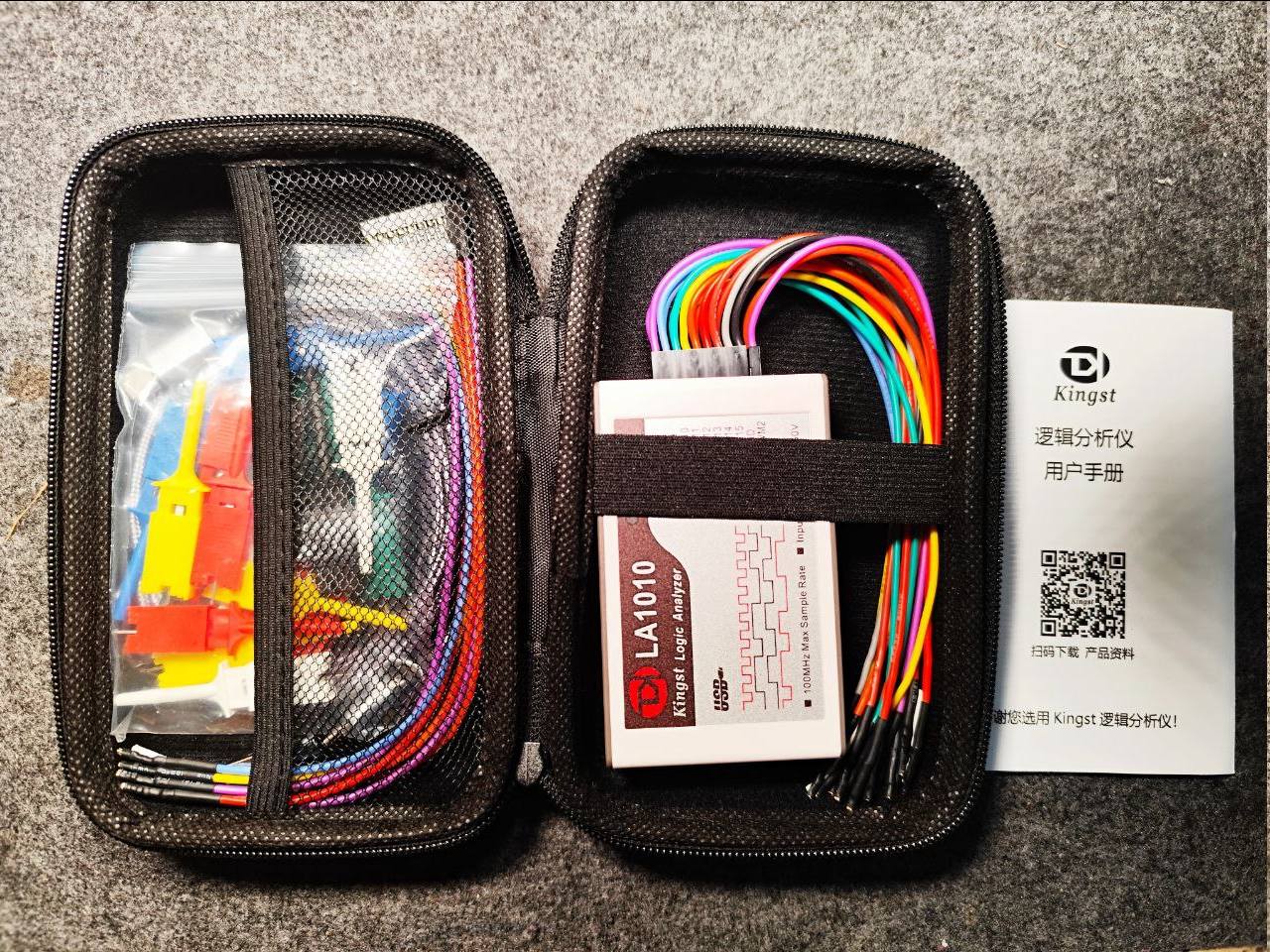
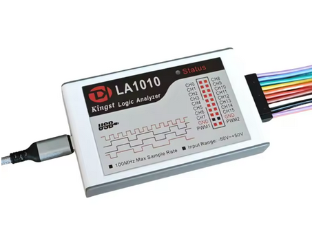
Received the 16-channel logic analyzer
10/23/2025 at 13:57 • 0 commentsAnother small step forward in the project: I’ve (quickly) received my 16-channel logic analyzer! The package and the box look nice.
It will allow me to observe the behavior at the FPGA pipeline output and check the signal synchronization.
No more hardware excuses for not moving forward… -
Reflections on FIR Filter Architecture
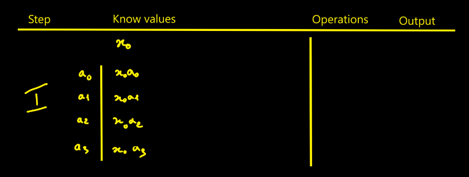
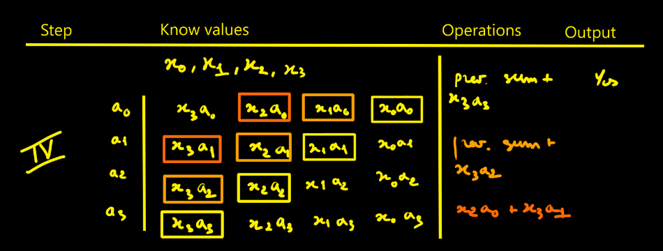
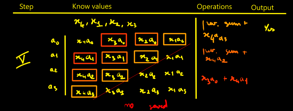
10/18/2025 at 14:53 • 0 commentsI thought designing the FIR filter would be simpler - in fact it isn’t that straightforward. To picture how data flows through the filter, I drew tables showing successive cycles with the propagation of values and the operations done at each step. The filter parameters are noted ai. The data to process are xi. Here we choose N = 4 for illustration.
I started with a direct approach, the way you’d do it on an MCU. You’ll see it’s probably not the right method here.
Per modulus mi, the FIR is:
yi[n] = ( Σk=0…N−1 hi[k] · xi[n−k] ) mod mi, for all i in [1, p]Reconstruction by CRT:
y[n] = CRT( y1[n], y2[n], …, yp[n] )To escape purely sequential thinking, it helps to reason in terms of a production line: separate “lines” manipulate data items, cycle after cycle, as in a factory.
Moreover I count the operations and accumulations involved in an FIR with N taps and it easier to do with the following tables:- N−1 additions
- N multiplications
- N cycles of latency (here one “cycle” means the time to ingest one full sample into the FPGA. The input sample is 16-bit, the input bus is 8-bit, so it takes 2 clocks to advance one cycle.)
- Looking at the step-5 table, we need to realize N + (N−1) + (N−2) + … + 1 = N(N+1)/2 intermediate products to fill the pipeline.
- We need to keep N products
- We also need to keep N−1 partial sums (accumulators)
Step-by-step
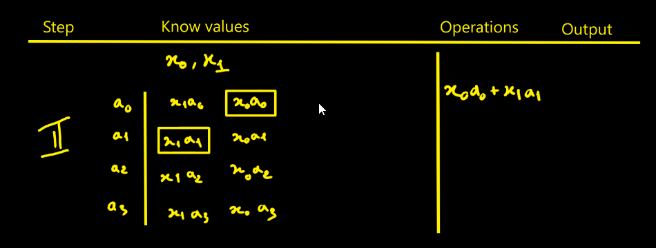
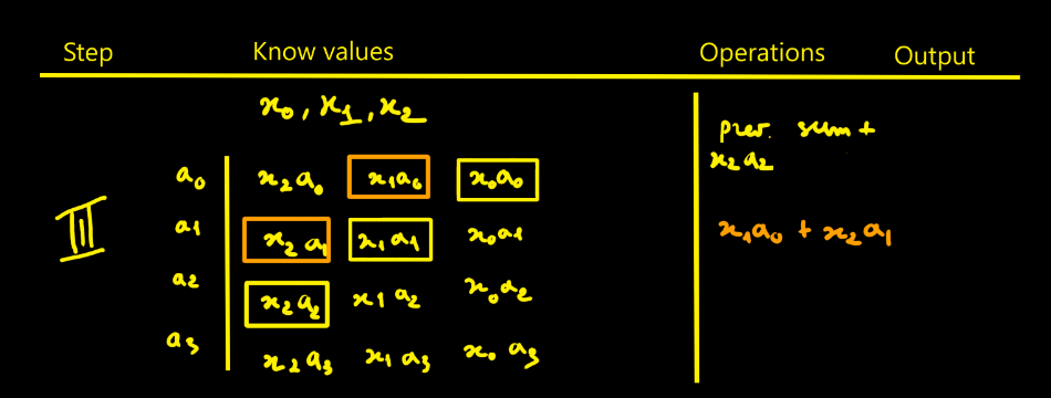
Figure 1. With x0 ingested, compute the four products tied to the filter {a0, a1, a2, a3}. Figure 2. When x1 arrives, compute its four products and start summing: x0a0 + x1a1. Figure 3. Ingest x2, add the new term x2a2 into the highlighted box. Start a new accumulator with x2a1 + x1a0. One more addition is still missing to complete a full convolution cycle. Figure 4. First full cycle completed: we can extract the first valid output. Figure 5. Continue the process. Values like x1a1, x1a2, x1a3, x2a2, etc., are not kept. A red boundary in the step-5 table marks what must be stored vs. what can be discarded. This is the direct approach. Of course, you must replicate that whole pipeline for each modulus. With k moduli, you duplicate it k times — that’s exactly where RNS parallelism comes from.
From the direct form to parallel and transposed architectures
While analyzing the cycle-by-cycle behavior of the direct form through these tables, a structural issue appears: for an FIR of N taps, the pipeline must effectively include N differentiated phases. At each cycle, every coefficient must be paired with its corresponding delayed sample — which requires a time-varying addressing scheme within the delay line.
As a result, the pipeline is not stationary: its internal data paths evolve from one cycle to the next (with a global sequence of N cycles). This makes programmation and sequencing heavier.
In addition to this non-stationary addressing, the addition chain itself must be broken into multiple intermediate stages to meet timing constraints. Together, these factors make the pipeline hard to program and tune.
Hence the natural question: isn’t there a more regular structure, where each pipeline stage would perform exactly the same operation at every instant?
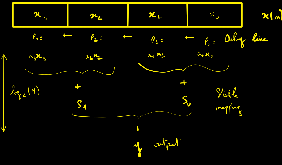
Parallel direct form (fully parallel direct FIR)
If one wants a “hard” (stationary) pipeline, the solution is to let the samples slide through a delay line:
X₃ ← X₂ ← X₁ ← X₀ ← x[n].The multipliers always see the correct positions (x[n], x[n−1], x[n−2], …): no more dynamic addressing.
![]()
That’s much better — but there’s still a hard point:
- the reduction of N products (modular addition tree) must itself be pipelined;
- otherwise, the final addition becomes heavy and limits fmax.
Pipelining this reduction introduces a few extra cycles of latency. In practice, if one addition combines two values, the reduction tree has log₂(N) stages. With a ternary adder (three inputs), this drops to roughly log₃(N).
This approach is scalable for frequency if the addition tree is balanced and pipelined (depth ≈ log₂ N). Ressources needed linear growth (N multipliers, ~N additions, and delay-line registers).
This approach is often preferred for large filters: short pipeline latency (≈ log₂ N), easy routing (tree fan-in), and a fully stationary structure.
Transposed pipeline (transposed / systolic form)
Another possible structure is the transposed form. It consists of a chain of identical cells, each performing a multiply–add (mod) operation followed by a register. In this configuration, every stage executes the same operation at each clock cycle, making the pipeline extremely regular. Once the pipeline is primed, it delivers one output per cycle (the same for parallel direct form) and typically achieves a very high operating frequency for small to medium filter sizes.
We reuse the same setup with N = 4 coefficients {a0, a1, a2, a3}.
In the transposed form, the input sample x[n] is broadcast to all four multipliers. Each cell performs a multiply–add (mod mi) followed by a register that stores the running sum for the next cycle.The internal registers are R1, R2, and R3. All operations below are taken mod mi.
y[n]  = a₀·x[n] + R1
R1'   = a₁·x[n] + R2
R2'   = a₂·x[n] + R3
R3'   = a₃·x[n]
After four cycles the pipeline is primed; from then on, one valid output is produced at every clock cycle. Each stage repeats the same operation at every cycle, which keeps timing and routing highly regular.
However, as N increases, a technological limitation appears: the input sample x[n] must be broadcast to all N multipliers in parallel. This high fan-out can degrade both fmax and routing quality unless the distribution network is segmented or pipelined.
In contrast, the parallel direct form only feeds x[n] into the first register of the delay line, and the data then propagates by simple shifting—an architecture that scales much more gracefully for large N.
RNS context — and my choice
Since my goal is to exploit the Residue Number System (RNS) to push dynamic range and build deep FIR filters (large N), the RNS approach shows its full advantage when the filter depth is high.
For the next steps of this project, I will therefore focus on the fully parallel direct form: it offers a short pipeline latency, routing better suited to large N (no massive fan-out at input), and a stationary pipeline structure.
In the next log, I’ll present the implementation for the parallel direct approach with N = 64.
-
From 8-bit Demo to Full RNS Pipeline: +2 Across 2^37 Dynamic Range
10/17/2025 at 09:42 • 0 commentsThis marks one of the key milestones towards the final objective: a design that performs +2, but this time using all 9 moduli, allowing for a dynamic range of 237.
Input data arrives via an 8-bit bus, in two cycles per word, while output data is mapped to 16 pins.
You can find the program on my github : https://github.com/Bertrand-selvasystems/rns-pipeline-16bitProgram Details (What Changed)
Data Capture, Phase 1
Input data enters the FPGA over an 8-bit bus. On each cycle, we alternately load the low and high bytes: the first byte received (LSB) is stored temporarily, then the next one (MSB) completes the 16-bit word. As soon as the word is complete, a one-cycle validity pulse (
v0) is issued to signal "word ready" for the next pipeline phase.
This simple handshake (in_fire = in_valid & in_ready, within_ready = rst_n) ensures the input is always ready (except during reset), simplifying both testbenches and real use.// Phase 1 — Capture 16b from 8b bus (LSB then MSB) reg [7:0] x_lo; reg have_lo; // 1 = LSB already captured reg v0; // 1-cycle pulse: 16b word ready reg [15:0] x0_16; wire in_fire = in_valid & in_ready; assign in_ready = rst_n; always @(posedge clk) begin if (!rst_n) begin have_lo <= 1'b0; v0 <= 1'b0; x_lo <= 8'd0; x0_16 <= 16'd0; end else begin v0 <= 1'b0; // default: no pulse if (in_fire) begin if (!have_lo) begin // First byte: LSB x_lo <= in_byte; have_lo <= 1'b1; end else begin // Second byte: MSB -> complete word + v0 pulse x0_16 <= {in_byte, x_lo}; have_lo <= 1'b0; v0 <= 1'b1; // **1-cycle pulse** end end end endOn each cycle when
in_fireis true:- If
have_lois 0, we capture the LSB. - If
have_lois 1, we capture the MSB, assemble the 16-bit word, and issuev0.
This mechanism guarantees no data is lost, and every incoming byte is processed at the rate dictated by the bus and module availability.
If you later want to handle discontinuous or asynchronous sources, simply make
in_readydependent on an actual FIFO or on the real buffering capacity of the module.In short: two input bytes come in, one 16-bit word goes out, marked by
v0for pipeline synchronization.Variable roles:
x_lo: temporary register for the first received byte (LSB).
have_lo: flag (1 bit) indicating whether the LSB has already been captured, controlling alternation between LSB storage and word assembly.
x0_16: register assembling the complete 16-bit word from the newly received MSB and the stored LSB.
v0: 1-cycle validity pulse; signals thatx0_16now holds a valid word ready for downstream processing.
in_fire: combinational signal that indicates a data transfer is happening this cycle (in_valid & in_ready).
in_ready: input availability signal; here, always 1 (except during reset), meaning the module never stalls the input—this is ideal for bench testing.Principle: On each
in_fire, if no LSB is present, we store the LSB inx_loand sethave_loto 1.
On the nextin_fire, the MSB is received, we assemble the 16-bit word intox0_16, resethave_loto 0, andv0emits a one-cycle pulse to signal "word ready".
This ensures lossless, overlap-free reconstruction, and maintains correct synchronization with the downstream pipeline.RNS to Binary Conversion, Phase 4
Here, we work with 9 coprime moduli (7, 11, 13, 15, 17, 19, 23, 29, 31), yielding a 37-bit dynamic range (M = 100,280,245,065). Reconstruction using the Chinese Remainder Theorem (CRT) is performed through weighted accumulation: each residue (ri) is assigned a value read from a precomputed ROM table (
T), and these terms are summed in multiple pipeline stages, each with a reduction modulo M.// Phase 4 — Pipelined CRT "mod M" at each addition stage localparam [36:0] M = 37'd100280245065; // Modular addition: returns (a+b) mod M function [36:0] add_modM; input [36:0] a, b; reg [37:0] s; // 0..(2*M-2) < 2^38 begin s = {1'b0,a} + {1'b0,b}; if (s >= {1'b0,M}) s = s - {1'b0,M}; add_modM = s[36:0]; end endfunction // ---- 4a: ROMs T* -> registers (37b) ---- reg v3a; reg [36:0] T7_r, T11_r, T13_r, T15_r, T17_r, T19_r, T23_r, T29_r, T31_r; always @(posedge clk) begin if (!rst_n) begin v3a<=1'b0; T7_r<=0; T11_r<=0; T13_r<=0; T15_r<=0; T17_r<=0; T19_r<=0; T23_r<=0; T29_r<=0; T31_r<=0; end else begin v3a <= v2; if (v2) begin T7_r <= T7 (r7p ); T11_r <= T11(r11p); T13_r <= T13(r13p); T15_r <= T15(r15p); T17_r <= T17(r17p); T19_r <= T19(r19p); T23_r <= T23(r23p); T29_r <= T29(r29p); T31_r <= T31(r31p); end end end // ---- 4b: level 1 (pairwise) -> registers (37b) ---- reg v3b; reg [36:0] L1a, L1b, L1c, L1d, L1e; always @(posedge clk) begin if (!rst_n) begin v3b<=1'b0; L1a<=0; L1b<=0; L1c<=0; L1d<=0; L1e<=0; end else begin v3b <= v3a; if (v3a) begin L1a <= add_modM(T7_r , T11_r); L1b <= add_modM(T13_r, T15_r); L1c <= add_modM(T17_r, T19_r); L1d <= add_modM(T23_r, T29_r); L1e <= T31_r; // single branch end end end // ---- 4c: level 2 -> registers (37b) ---- reg v3c; reg [36:0] L2a, L2b, L2e; always @(posedge clk) begin if (!rst_n) begin v3c<=1'b0; L2a<=0; L2b<=0; L2e<=0; end else begin v3c <= v3b; if (v3b) begin L2a <= add_modM(L1a, L1b); L2b <= add_modM(L1c, L1d); L2e <= L1e; // pipeline alignment end end end // ---- 4d: (L2a + L2b) mod M -> register -------- reg v4; reg [36:0] S4_mod; reg [15:0] y4; reg v3d; reg [36:0] sum_ab; always @(posedge clk) begin if (!rst_n) begin v3d <= 1'b0; sum_ab<= 37'd0; end else begin v3d <= v3c; if (v3c) sum_ab <= add_modM(L2a, L2b); end end // ---- 4e: (sum_ab + L2e) mod M -> S4_mod / y4 ---- wire [36:0] S4_mod_next = add_modM(sum_ab, L2e); always @(posedge clk) begin if (!rst_n) begin v4 <= 1'b0; S4_mod <= 37'd0; y4 <= 16'd0; end else begin v4 <= v3d; // validity alignment if (v3d) begin S4_mod <= S4_mod_next; y4 <= S4_mod_next[15:0]; end end endEach pipeline stage is a modular addition, followed by a register and a validity bit. We start by reading the CRT terms in parallel from the ROMs, then reduce them in an adder tree: 4b (9→5), 4c (5→3), 4d (3→2), and finally 4e (final output), all synchronized at every cycle. The tree structure breaks the critical path: instead of one huge 9-term adder (which limited Fmax to 56 MHz), the sum is decomposed into smaller, pipelined adders, pushing Fmax up to 109 MHz (post-synthesis Quartus).
The validity bits (
v3a, v3b, v3c, v3d, v4) act as a “breadcrumb trail”: at each stage, they guarantee that data is always correctly aligned, never mixing samples.Memory usage remains modest: for 9 moduli, each CRT table is
m_ientries × 37 bits, for a total of 165 × 37 = 6,105 bits (<1 kB), plus about 2.5 kB for the binary→RNS conversion. Overall, the design fits comfortably within less than 3.5 kB of on-chip RAM.Results
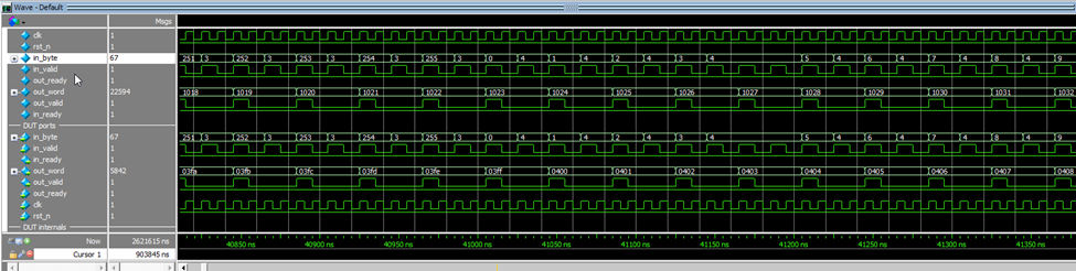
The simulation capture above shows the pipeline processing a stream of 16-bit words, each received as two bytes (LSB then MSB). Each word is reconstructed as soon as the second byte arrives, processed through the entire RNS chain, and then output after a fixed delay. For each injected word (e.g., the pair 254/3, i.e., 0x03FE), the output delivers the expected result (here 0x0400, i.e., 1022+2 modulo 16 bits). Input and output handshakes are tightly paced: the input is always ready, and the output publishes one result per pipeline “tick.”
In terms of latency, there are exactly eight clock cycles from receiving the MSB to the output result — corresponding to the pipeline depth (all internal stages propagate in 8 clock cycles). In practice, the module runs at the input stream’s cadence, with maximal throughput determined by byte feeding rate (here, one word every two cycles due to the 8-bit input bus).
Bottom line: it works. It does +2 — it’s admittedly heavy for just a +2, but it’s a full proof of concept. There’s no duplication or data loss. It counts to 65,000 in under 2ms, one word every 20ns… Real-world hardware testing will follow.
These results show that the entire pipeline, including the modular operations, binary→RNS conversion, and final RNS→binary conversion, is functioning correctly (no errors in the LUTs or the conversions).
Rest of the Design
The rest of the code closely resembles the 8-bit case. The structure is identical, but the precomputed tables are more numerous and larger, resulting in a total memory footprint of about 3.5 kB.
Outlook and Technical Comments
There are two major steps left before this project is “feature complete,” per the initial spec. This topic is, to me, genuinely interesting. It may enable truly low-cost, low-energy signal processing — but only for “fixed pipeline” architectures: comparisons and non-linear operations (especially divisions) are heavy in RNS, but for FIR, time-domain correlation, and similar tasks, RNS is a strong candidate when you need massive dynamic range.
Additionally, RNS offers a natural path to redundancy, thanks to its inherently parallel structure. In any context where error management is critical, this could open new opportunities.
But here, the objectives remain simple:- Replace the “+2” with a functional FIR filter of 64 or 128 elements.
- Wire up the hardware to a real ESP32 and observe real-world behavior.
For hardware testing, I purchased this 16-input logic analyzer to observe the 16-bit output bus directly (50€ for 100 Mhz). The 8-bit input stream will be generated by the ESP32.
- If
-
Automatic Generation of RNS LUTs in MATLAB
10/16/2025 at 09:02 • 0 commentsThis MATLAB/Octave script automatically computes look-up tables (LUTs) for a Residue Number System (RNS) with a given set of moduli. It generates:
- The total product
M = m1 * m2 * ... * mn - The reconstruction coefficients
Ai - An example table
Tjfor a modulusmj - Verilog-style outputs (
case / endcase) ready to integrate into your FPGA design
Method
The reconstruction follows the classical Chinese Remainder Theorem (CRT):
M  = product of all moduli
Mi = M / mi
Ai = (Mi * inverse(Mi mod mi, mi)) mod M
Tm(r) = (Ai * r) mod M   for r = 0 .. mi-1
Each
Tmtable stores precomputed modular residues, allowing fast RNS operations on FPGA without any division or modulo logic.MATLAB/OCTAVE Script
close all;
clear all;
clc;
format long g;

%% RNS LUT generation

%% Moduli list
moduli = [7 11 13 15 17 19 23 29 31];

%% Compute M
M = 1;
for i = 1:length(moduli)
    M = M * moduli(i);
end
disp(M);   % 100280245065

%% Coefficients Ai
Ai = zeros(1, numel(moduli));   % preallocation
for i = 1:numel(moduli)
    m  = moduli(i);
    Mi = M / m;                 % M_i
    t  = mod(Mi, m);            % (M_i mod m)
    [g, x, ~] = gcd(t, m);      % t*x + m*y = g
    if g ~= 1
        error('No modular inverse for m=%d (gcd=%d).', m, g);
    end
    inv_t = mod(x, m);          % inverse of t modulo m
    Ai(i) = mod(inv_t * Mi, M); % A_i = (M_i * inv_t) mod M
end

%% Example LUT Tj (e.g., j=9 -> m = 31)
j  = 9;                         % choose index in 'moduli'
mj = moduli(j);
Tj = zeros(1, mj);              % Tj(r+1) = (Ai(j)*r) mod M

for r = 0 : mj-1
    Tj(r+1) = mod(Ai(j) * r, M);
end

% Display
disp('Ai ='); disp(Ai);
disp(['T' num2str(mj) '(r) for r=0..' num2str(mj-1) ':']);
disp(Tj);

%% Verilog-like table generator
for j = 1:numel(moduli)
    m = moduli(j);
    fprintf('function [36:0] T%d;\n', m);
    fprintf('  input [4:0] r;\n  begin\n    case (r)\n');
    for r = 0:m-1
        fprintf('      5''d%-2d : T%d = 37''d%u;\n', r, m, mod(Ai(j)*r,M));
    end
    fprintf('      default: T%d = 37''d0;\n    endcase\n  end\nendfunction\n\n', m);
end
Notes
- Chosen moduli:
[7, 11, 13, 15, 17, 19, 23, 29, 31] - Total product: M = 100,280,245,065
- Because
2^37 = 137,438,953,472 > M, 37-bit wide signals are sufficient. - Each input
rfits in 5 bits (max modulus = 31). - In this configuration, M is large enough to prevent overflow when using Q15 coefficients in an RNS-based FIR filter (the goal project).
Conclusion
This log automates the generation of RNS LUTs and Verilog snippets. Run the script, copy the output, and integrate it directly into your FPGA design without manual editing. Because Typing 300 Constants by Hand Is for Humans...
Results
function [36:0] T7;
input [4:0] r;
begin
case (r)
5'd0 : T7 = 37'd0;
5'd1 : T7 = 37'd28651498590;
5'd2 : T7 = 37'd57302997180;
5'd3 : T7 = 37'd85954495770;
5'd4 : T7 = 37'd14325749295;
5'd5 : T7 = 37'd42977247885;
5'd6 : T7 = 37'd71628746475;
default: T7 = 37'd0;
endcase
end
endfunctionfunction [36:0] T11;
input [4:0] r;
begin
case (r)
5'd0 : T11 = 37'd0;
5'd1 : T11 = 37'd91163859150;
5'd2 : T11 = 37'd82047473235;
5'd3 : T11 = 37'd72931087320;
5'd4 : T11 = 37'd63814701405;
5'd5 : T11 = 37'd54698315490;
5'd6 : T11 = 37'd45581929575;
5'd7 : T11 = 37'd36465543660;
5'd8 : T11 = 37'd27349157745;
5'd9 : T11 = 37'd18232771830;
5'd10 : T11 = 37'd9116385915;
default: T11 = 37'd0;
endcase
end
endfunctionfunction [36:0] T13;
input [4:0] r;
begin
case (r)
5'd0 : T13 = 37'd0;
5'd1 : T13 = 37'd53997055035;
5'd2 : T13 = 37'd7713865005;
5'd3 : T13 = 37'd61710920040;
5'd4 : T13 = 37'd15427730010;
5'd5 : T13 = 37'd69424785045;
5'd6 : T13 = 37'd23141595015;
5'd7 : T13 = 37'd77138650050;
5'd8 : T13 = 37'd30855460020;
5'd9 : T13 = 37'd84852515055;
5'd10 : T13 = 37'd38569325025;
5'd11 : T13 = 37'd92566380060;
5'd12 : T13 = 37'd46283190030;
default: T13 = 37'd0;
endcase
end
endfunctionfunction [36:0] T15;
input [4:0] r;
begin
case (r)
5'd0 : T15 = 37'd0;
5'd1 : T15 = 37'd6685349671;
5'd2 : T15 = 37'd13370699342;
5'd3 : T15 = 37'd20056049013;
5'd4 : T15 = 37'd26741398684;
5'd5 : T15 = 37'd33426748355;
5'd6 : T15 = 37'd40112098026;
5'd7 : T15 = 37'd46797447697;
5'd8 : T15 = 37'd53482797368;
5'd9 : T15 = 37'd60168147039;
5'd10 : T15 = 37'd66853496710;
5'd11 : T15 = 37'd73538846381;
5'd12 : T15 = 37'd80224196052;
5'd13 : T15 = 37'd86909545723;
5'd14 : T15 = 37'd93594895394;
default: T15 = 37'd0;
endcase
end
endfunctionfunction [36:0] T17;
input [4:0] r;
begin
case (r)
5'd0 : T17 = 37'd0;
5'd1 : T17 = 37'd17696513835;
5'd2 : T17 = 37'd35393027670;
5'd3 : T17 = 37'd53089541505;
5'd4 : T17 = 37'd70786055340;
5'd5 : T17 = 37'd88482569175;
5'd6 : T17 = 37'd5898837945;
5'd7 : T17 = 37'd23595351780;
5'd8 : T17 = 37'd41291865615;
5'd9 : T17 = 37'd58988379450;
5'd10 : T17 = 37'd76684893285;
5'd11 : T17 = 37'd94381407120;
5'd12 : T17 = 37'd11797675890;
5'd13 : T17 = 37'd29494189725;
5'd14 : T17 = 37'd47190703560;
5'd15 : T17 = 37'd64887217395;
5'd16 : T17 = 37'd82583731230;
default: T17 = 37'd0;
endcase
end
endfunctionfunction [36:0] T19;
input [4:0] r;
begin
case (r)
5'd0 : T19 = 37'd0;
5'd1 : T19 = 37'd58056983985;
5'd2 : T19 = 37'd15833722905;
5'd3 : T19 = 37'd73890706890;
5'd4 : T19 = 37'd31667445810;
5'd5 : T19 = 37'd89724429795;
5'd6 : T19 = 37'd47501168715;
5'd7 : T19 = 37'd5277907635;
5'd8 : T19 = 37'd63334891620;
5'd9 : T19 = 37'd21111630540;
5'd10 : T19 = 37'd79168614525;
5'd11 : T19 = 37'd36945353445;
5'd12 : T19 = 37'd95002337430;
5'd13 : T19 = 37'd52779076350;
5'd14 : T19 = 37'd10555815270;
5'd15 : T19 = 37'd68612799255;
5'd16 : T19 = 37'd26389538175;
5'd17 : T19 = 37'd84446522160;
5'd18 : T19 = 37'd42223261080;
default: T19 = 37'd0;
endcase
end
endfunctionfunction [36:0] T23;
input [4:0] r;
begin
case (r)
5'd0 : T23 = 37'd0;
5'd1 : T23 = 37'd87200213100;
5'd2 : T23 = 37'd74120181135;
5'd3 : T23 = 37'd61040149170;
5'd4 : T23 = 37'd47960117205;
5'd5 : T23 = 37'd34880085240;
5'd6 : T23 = 37'd21800053275;
5'd7 : T23 = 37'd8720021310;
5'd8 : T23 = 37'd95920234410;
5'd9 : T23 = 37'd82840202445;
5'd10 : T23 = 37'd69760170480;
5'd11 : T23 = 37'd56680138515;
5'd12 : T23 = 37'd43600106550;
5'd13 : T23 = 37'd30520074585;
5'd14 : T23 = 37'd17440042620;
5'd15 : T23 = 37'd4360010655;
5'd16 : T23 = 37'd91560223755;
5'd17 : T23 = 37'd78480191790;
5'd18 : T23 = 37'd65400159825;
5'd19 : T23 = 37'd52320127860;
5'd20 : T23 = 37'd39240095895;
5'd21 : T23 = 37'd26160063930;
5'd22 : T23 = 37'd13080031965;
default: T23 = 37'd0;
endcase
end
endfunctionfunction [36:0] T29;
input [4:0] r;
begin
case (r)
5'd0 : T29 = 37'd0;
5'd1 : T29 = 37'd41495273820;
5'd2 : T29 = 37'd82990547640;
5'd3 : T29 = 37'd24205576395;
5'd4 : T29 = 37'd65700850215;
5'd5 : T29 = 37'd6915878970;
5'd6 : T29 = 37'd48411152790;
5'd7 : T29 = 37'd89906426610;
5'd8 : T29 = 37'd31121455365;
5'd9 : T29 = 37'd72616729185;
5'd10 : T29 = 37'd13831757940;
5'd11 : T29 = 37'd55327031760;
5'd12 : T29 = 37'd96822305580;
5'd13 : T29 = 37'd38037334335;
5'd14 : T29 = 37'd79532608155;
5'd15 : T29 = 37'd20747636910;
5'd16 : T29 = 37'd62242910730;
5'd17 : T29 = 37'd3457939485;
5'd18 : T29 = 37'd44953213305;
5'd19 : T29 = 37'd86448487125;
5'd20 : T29 = 37'd27663515880;
5'd21 : T29 = 37'd69158789700;
5'd22 : T29 = 37'd10373818455;
5'd23 : T29 = 37'd51869092275;
5'd24 : T29 = 37'd93364366095;
5'd25 : T29 = 37'd34579394850;
5'd26 : T29 = 37'd76074668670;
5'd27 : T29 = 37'd17289697425;
5'd28 : T29 = 37'd58784971245;
default: T29 = 37'd0;
endcase
end
endfunctionfunction [36:0] T31;
input [4:0] r;
begin
case (r)
5'd0 : T31 = 37'd0;
5'd1 : T31 = 37'd16174233075;
5'd2 : T31 = 37'd32348466150;
5'd3 : T31 = 37'd48522699225;
5'd4 : T31 = 37'd64696932300;
5'd5 : T31 = 37'd80871165375;
5'd6 : T31 = 37'd97045398450;
5'd7 : T31 = 37'd12939386460;
5'd8 : T31 = 37'd29113619535;
5'd9 : T31 = 37'd45287852610;
5'd10 : T31 = 37'd61462085685;
5'd11 : T31 = 37'd77636318760;
5'd12 : T31 = 37'd93810551835;
5'd13 : T31 = 37'd9704539845;
5'd14 : T31 = 37'd25878772920;
5'd15 : T31 = 37'd42053005995;
5'd16 : T31 = 37'd58227239070;
5'd17 : T31 = 37'd74401472145;
5'd18 : T31 = 37'd90575705220;
5'd19 : T31 = 37'd6469693230;
5'd20 : T31 = 37'd22643926305;
5'd21 : T31 = 37'd38818159380;
5'd22 : T31 = 37'd54992392455;
5'd23 : T31 = 37'd71166625530;
5'd24 : T31 = 37'd87340858605;
5'd25 : T31 = 37'd3234846615;
5'd26 : T31 = 37'd19409079690;
5'd27 : T31 = 37'd35583312765;
5'd28 : T31 = 37'd51757545840;
5'd29 : T31 = 37'd67931778915;
5'd30 : T31 = 37'd84106011990;
default: T31 = 37'd0;
endcase
end
endfunction - The total product
-
Receiving the USB Blaster
10/14/2025 at 14:17 • 0 commentsI just received the Altera USB Blaster, used to program the Cyclone IV FPGA.
What it’s for:
-
JTAG interface between the PC and Intel/Altera FPGA or CPLD (Cyclone, MAX, etc.)
-
Programming of configuration files (.sof, .pof, .jic) via Quartus
-
Hardware debugging access (SignalTap, JTAG UART, boundary-scan)
-
Low-level memory read/write and diagnostic operations
The real tests will begin soon. I’ll post a log once the first successful programming sequence is done.
![]()
-
Winter, FPGAs, and Forgotten Arithmetic
RNS on FPGA: Revisiting an Unusual Number System for Modern Signal Processing

 At the same time, if I’d bought the 10-wire ribbon cable on its own, it would have cost me more than 2€. I don’t have the motivation to open it up and see what’s inside. But it’s definitely better to go for another model…
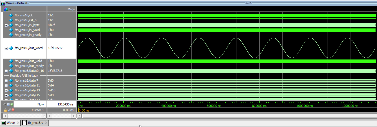

 The list of filter elements values :