JASPER : FTIR

We're back with an exciting update on our DIY Fourier-Transform Infrared (FTIR) project! It's time to put those white light fringes behind us and focus on capturing robust IR interferograms. Our goal is to use a pyroelectric detector, which means we need a reliable, powerful thermal source.

🔬 MEMS Emitter & Our Full ZnSe Optical Upgrade

Our initial approach used a MEMS IR emitter. It seemed ideal for its fast startup and simpler electronics, which could also be reused for future pulsed NDIR (Non-Dispersive Infrared) designs.

To properly work with mid-IR light, we made major optical changes:

• Full ZnSe Optics: The entire optical path—including the beam splitter, focusing, and collimation elements—is now made of Zinc Selenide (ZnSe).
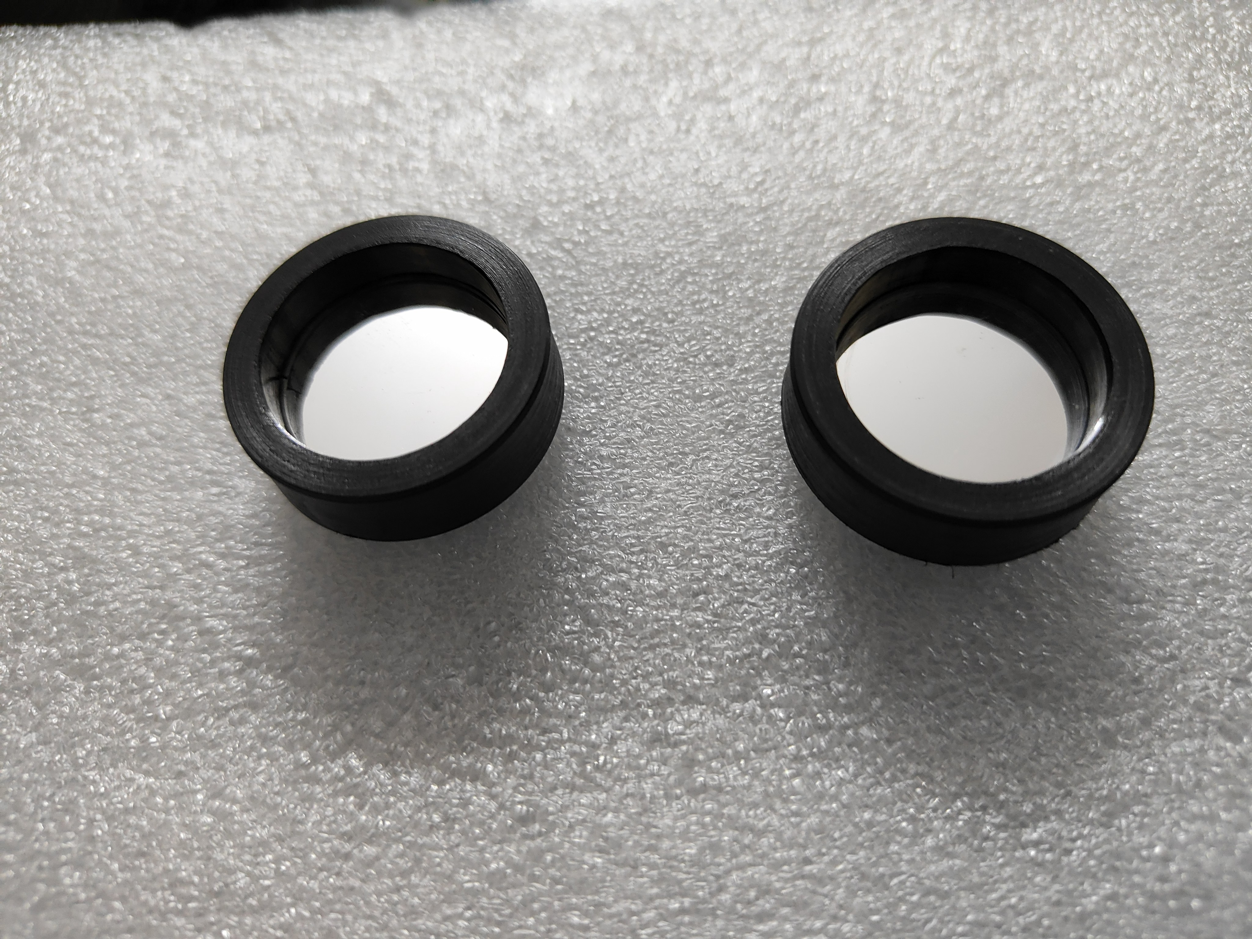
• Hollow Retroreflector: We replaced our standard retroreflector prism (made of BK7 glass, which would absorb the entire IR signal) with a hollow retroreflector. This ensures the IR radiation remains unimpeded.
  
• NIR Alignment: Since ZnSe is opaque to visible light, we switched our alignment source to a Near-Infrared (NIR) laser diode.
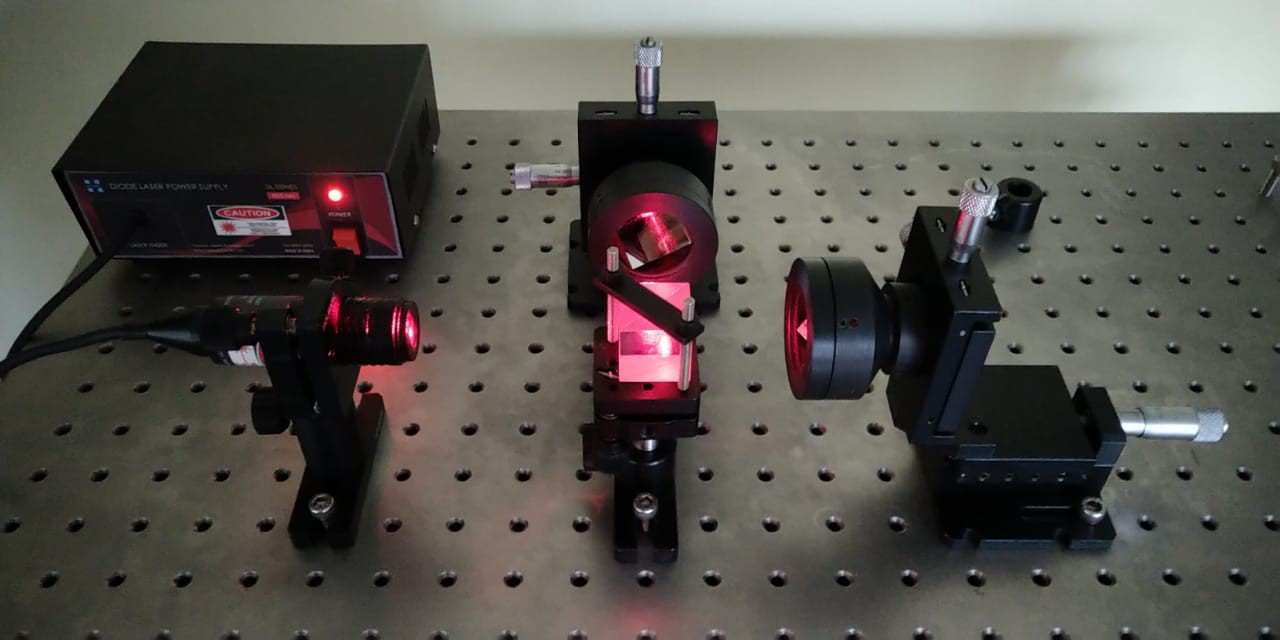
• Co-Axial Alignment: To merge the NIR laser and the IR light, we experimented with a mirror that had an elliptical center hole. Tilted at an angle, this created a circular aperture, bringing both sources onto the same optical axis.
• Verification: We used a thermal camera to visually confirm the presence of fringes, ensuring our alignment was correct before moving to the final pyroelectric detector.

We intentionally avoided expensive Off-Axis Parabolic (OAP) mirrors for this stage, focusing on validating the basic alignment necessary to capture IR fringes.

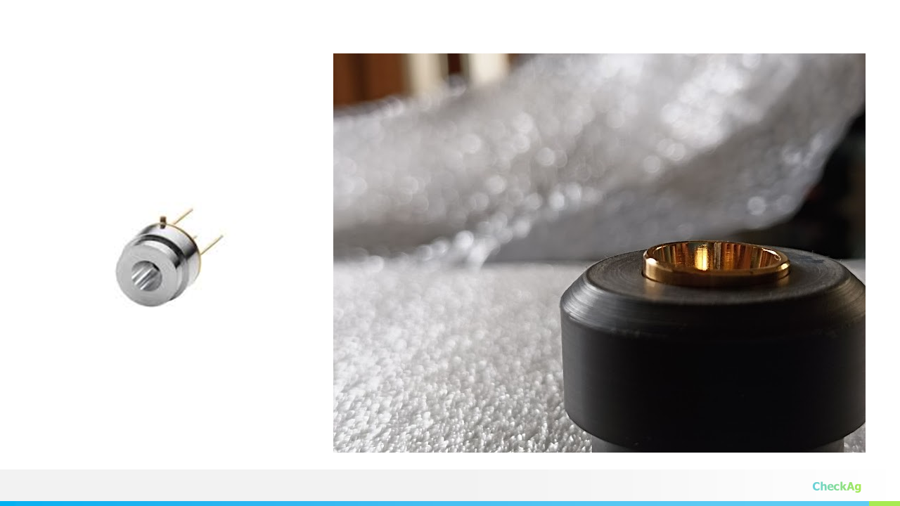
                                                                               MEMS Emitter  

                                                               Hollow Retroreflectors

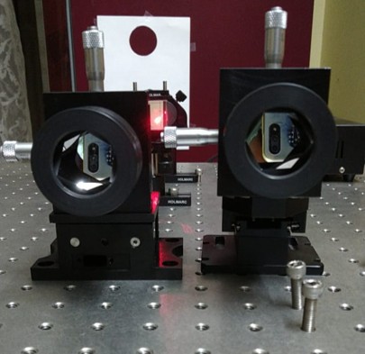
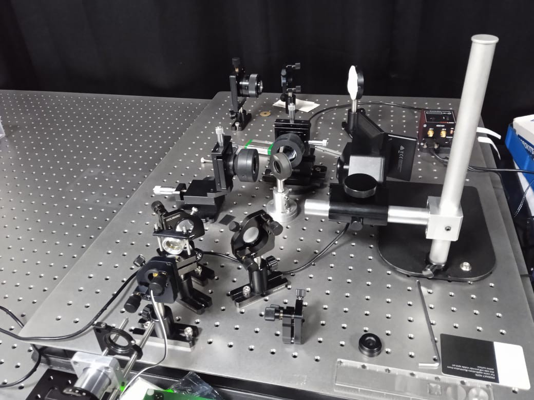
                                                  Initial Setup with MEMS IR emitter

💥 Catastrophic Failure and the Component Abuse Solution

The precise alignment was brutal, forcing us to run the MEMS IR emitter in continuous, constant-power mode for hours on end. Ultimately, the stress proved too much for the driver board, and it failed, leaving us without our critical light source.

We needed a replacement—fast and cheap! After considering alternatives like tungsten lamps, we stumbled upon the perfect hack that perfectly fits the component abuse spirit: a 3D printer heater cartridge.

Why a 3D Printer Cartridge Works Better

Replacement 3D printer heater cartridges are incredibly cheap and widely available. Though likely a Nickel-Chromium (Nichrome) alloy, the key advantage is the sheer power. Where the MEMS emitter offered minimal power, these cartridges are rated for 12V, 40W or 24V, 70W. For an FTIR, we actually need that increased thermal power for a higher signal.

We designed and printed a custom holder to swap out the failed MEMS unit for the cartridge. For now, driving it is simple: a DC bench power supply is all we need to get the heat for alignment. While we know the resistance increases with temperature (meaning an ideal design would have a constant power driver), the cartridge is a fantastic, high-power, temporary source.

This inexpensive part proved to be our savior, providing the thermal output needed to continue the project.

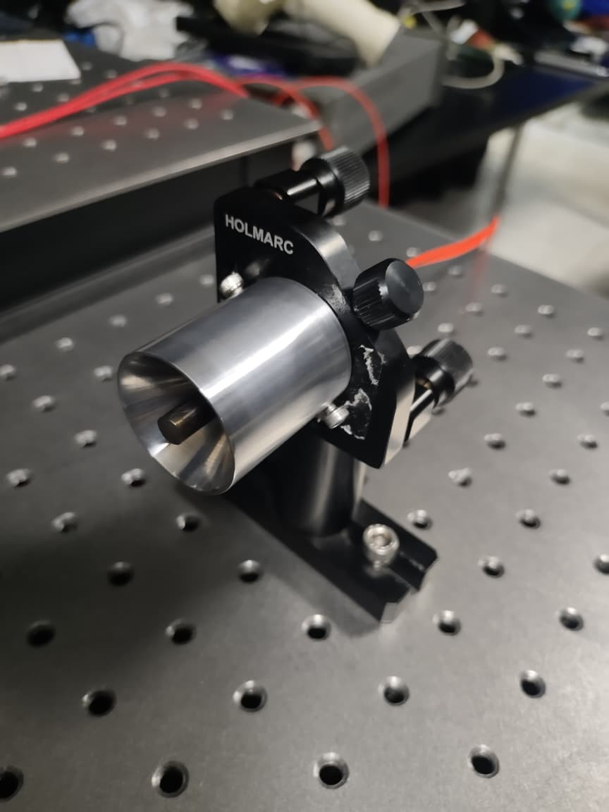
                                       IR Source with 3D Printer heater element 

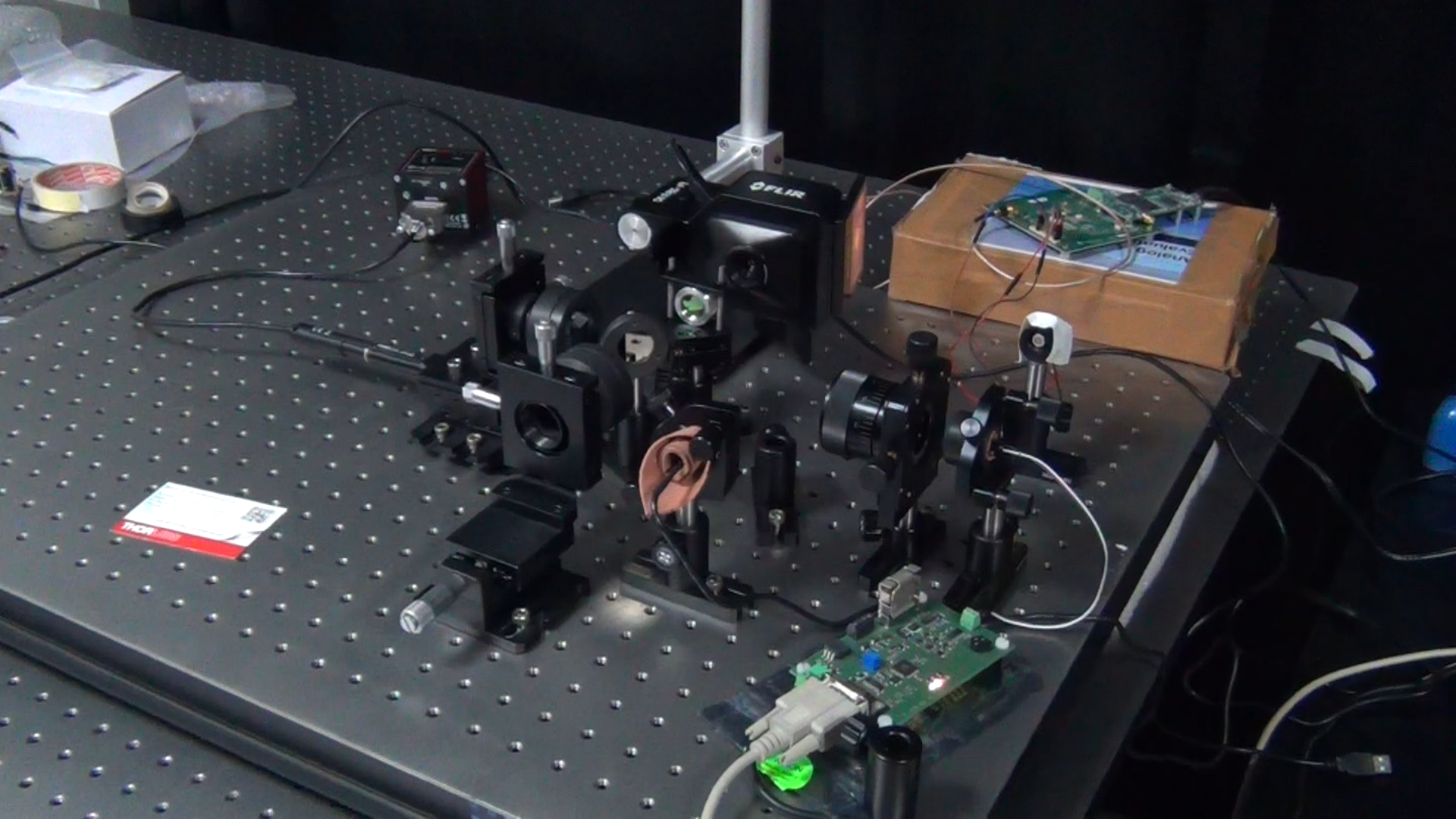
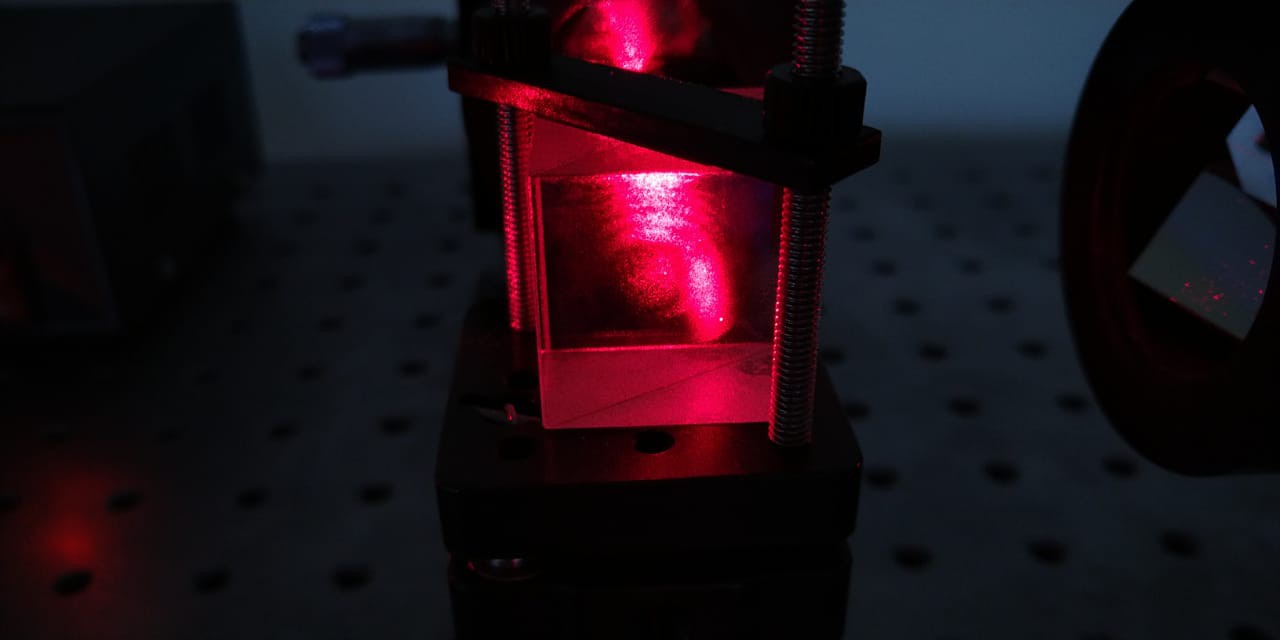
                                       One of Our Iterative Optical Configurations

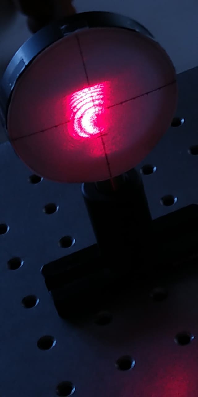
✨ Thermal Fringes Confirmed!

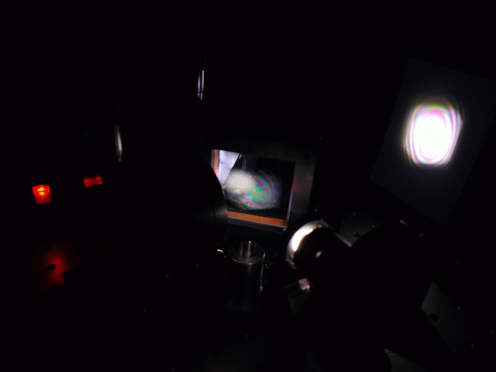
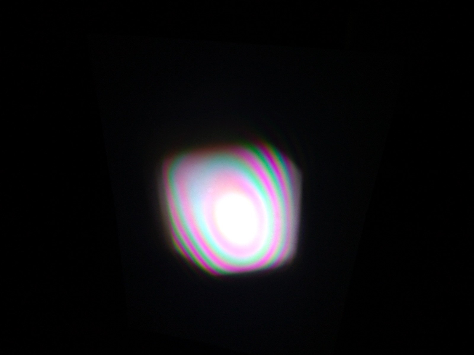
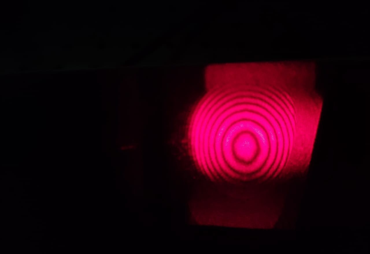
With the 3D printer heater cartridge in place, we successfully recorded the first thermal fringes using our FLIR thermal camera!

This beautiful thermal interferogram confirms our full ZnSe optics setup is aligned and working.

This success raises an intriguing question: Could an affordable thermal camera (a microbolometer, typically operating in 8-14µm region) be used as the actual detector for a budget spectrometer? While intriguing, for true FTIR resolution and speed, it's necessary to stick with specialized pyroelectric detectors like DLaTGS or LiTaO3. These offer a much smaller thermal time constant (critical for scanning mirrors) and cover the entire far-to-mid IR spectral range, ensuring the best possible interferogram quality.

Next Step: We'll dive into the math and software required for the Fourier Transform—the critical step that converts the spatial (or temporal) interferogram fringes into the final infrared absorption spectrum. We also need to start designing the electronics for the pyroelectric detector data acquisition system. More details on the transform and the hardware design are coming in the next posts!

We've all enjoyed the relatively simple beauty of laser interference fringes. Armed with a red or green laser diode and a basic Michelson Interferometer, fringes appear easily because of the laser’s high coherence length. Imperfect optics or slightly misaligned mirrors? No problem—the fringes are often still there!

Our current quest, however, is far more challenging: achieving interference fringes using a broadband white LED.

Coherence is King (and White Light is the Usurper)

Switching to a broadband source fundamentally changes the game. While a laser might have a coherence length measured in meters, a white LED’s is drastically shorter—often just a few micrometers (µm).

This is why the literature is spot-on: for white light fringes to occur, the path length difference between the two arms of the interferometer must be incredibly small. We're talking less than a micrometer of deviation (∆L < 1 µm) near the Zero Path Difference (ZPD) point.

🛠️ The Optics Challenge: From Planar Mirrors to Retroreflectors

Our initial attempts with standard planar mirrors were frustrating. It’s nearly impossible to ensure perfect parallelism and zero deviation with manual alignment and imperfect components. Even slight mirror imperfections, which a highly coherent laser shrugs off, completely destroy the faint white light fringes.

Our breakthrough came with retroreflectors (also known as corner-cube mirrors). These components, commonly found in commercial FTIR systems, inherently return the incoming beam parallel to itself, regardless of the retroreflector’s exact orientation (within limits). This stability proved critical for maintaining the necessary precision, allowing the light from both arms to recombine coherently, thereby addressing the high sensitivity of white light interference to angular alignment.

The Alignment Grind 📐

Perfect alignment is the ultimate hurdle. We’ve had to adopt a multi-step approach:

1. Laser Homing: We start by using a visible laser (like the red one) to generate fringes. We track the movement of the fringes as we move the mirror, mapping out the distance and locating the general region of the ZPD.
2. The Window & Beamsplitter: The compensation window and beamsplitter arrangement is crucial. To simplify alignment and guarantee parallelism, we’ve sandwiched the two components into a single, tightly enclosed assembly. This ensures that the beamsplitter’s thickness is perfectly compensated by the window, minimizing path errors caused by dispersion.
3. The White Light Moment: Only when the laser alignment is near-perfect do we switch to the white LED. The fringe pattern only appears for a minuscule movement of the mirror—literally a few micrometers.
4. The Target: We are aiming for perfect circular fringes , which signify that the interferometer is perfectly aligned and the two wavefronts are planar and parallel across the entire beam.

Sometimes, this process takes mere minutes; other times, it's an hours-long battle—truly a needle-in-a-haystack search for the Zero Path Difference.

Looking Ahead to the Invisible: FTIR Challenges

Our end goal is to work in the infrared (IR) spectrum for Fourier-Transform Infrared (FTIR) spectroscopy. This presents a new, major problem: we cannot see the IR fringes. We'll have to rely on thermal cameras or sensitive detectors.

In commercial FTIR systems, this is often handled by having a KBr beamsplitter, which is transparent to both visible (white) and IR light. Manufacturers align the ZPD using a visible white light source and then swap the source for the thermal IR emitter, knowing the alignment holds.

But with materials like ZnSe (often required for certain IR ranges), we lose that luxury, as ZnSe is opaque to visible light. We must devise a robust way to achieve perfect alignment and ZPD using only the IR source, or an ingenious external visible alignment reference.

White light interferometry is the core principle behind Fourier Transform Spectroscopy (FTS), which is dominant in the IR (FTIR) and Terahertz range. However, for the visible and UV spectrum, the extreme mechanical precision required to scan a tiny distance for broadband visible light and the computational overhead of the Fourier Transform generally make them less practical than robust grating systems.

You can view the video to see the perfect circular fringes we finally managed to capture using the white light LED. This pattern signifies the interferometer has reached the highest level of alignment and is a must-achieve milestone before we can move on to working with invisible infrared (IR) light.

When we switch to IR, we lose this valuable visual cue and will have to rely entirely on detectors or thermal cameras to "see" the fringes.

Why No White Light Spectrometers?

You might wonder why, given the successful demonstration of white light fringes, we don't see many white light interferometry-based spectrometers on the market.

The reason largely comes down to the maturity and performance of grating-based spectrometers.

• Simplicity and Robustness: Grating systems are mechanically simpler and more robust, without the ultra-precise, micrometer-level moving mirror requirement of an interferometer.
• Performance: Grating spectrometers offer excellent spectral resolution and throughput, making them the default choice.

Our journey continues as we search for that elusive "easy" way to achieve IR  ZPD! Stay tuned for more updates.

The Fourier-Transform Infrared (FTIR) spectrometer is an icon of analytical chemistry, offering incredible speed and high-resolution spectral data. Every classic FTIR relies on a Michelson interferometer, and at the core of its precision is a tiny, red Helium-Neon (HeNe) laser acting as the ultimate, unmoving yardstick.

But what happens when your project demands optics that block that trusty red light? We faced this exact problem using Zinc Selenide (ZnSe) optics for specialized IR range work. Since ZnSe is opaque to visible light, the 632.8nm HeNe beam is useless. We must switch to a Near-Infrared (NIR) diode laser, which brings a major headache: instability.

A diode laser's wavelength shifts dramatically with temperature and current fluctuations. If the "ruler" you're using to measure the mirror's position changes size mid-scan, your spectral data is useless. Here is the hack—a way to precisely measure an unknown, unstable wavelength by first using a second, known laser to perfectly map the mirror's movement.

The HeNe Foundation: Position is Everything

In FTIR, the entire analysis depends on the computer knowing the exact mirror displacement ∆x when the IR signal is sampled.

The HeNe laser achieves this by producing an interference signal ∆x that cycles with the distance moved:

Since the HeNe wavelength λ_HeNe = 632.8nm is stable and known to extreme precision, every single fringe (cycle) corresponds to a mirror movement of exactly λ_HeNe /2 ≈ 316.4 nm. This stability is why the HeNe has been the Grandfather of FTIR; it converts a noisy, unpredictable motor movement into a perfectly known, equidistant sampling grid.

🛠️ The DIY Calibration Hack: Two Lasers, One Ruler

To solve the unstable NIR diode problem, we introduce a known, stable reference laser (let's call it the Red Laser, λ_Red). We monitor this stable reference simultaneously with the unknown measurement laser to account for both motor speed variation and the diode's mid-scan wavelength drift.

This hack breaks the complex problem (Unknown λ and v) into two manageable steps.

Step 1: Establish the Perfect Ruler (Mirror Position)

The mirror's instantaneous velocity v is the primary unknown. We eliminate it by using the known, stable λ_Red signal.

1. Digitizing the Red Signal: We constantly monitor the fringes from the stable Red Laser with a dedicated detector.
2. Mapping Displacement: We count the time ∆t between two adjacent maxima (fringes) in the Red signal. This movement corresponds to a mirror displacement of exactly ∆x = λ_Red / 2.
3. Calculating Velocity (If Needed): While the ultimate goal is position, this process simultaneously reveals the instantaneous velocity: v = ∆x / ∆t

By tracking this process for every fringe, the digitized Red signal generates a high-precision, time-resolved map of the mirror's absolute position ∆x. Crucially, this position data is based only on the known λ_Red, making it independent of any motor speed instability.

Step 2: Calculate the Unknown Wavelength λ_Green

With the mirror's position precisely mapped by λ_Red, we can now use that map to determine the wavelength of the unstable measurement laser, λ_Green, from its simultaneously recorded fringe pattern.

1. Set a Distance: Define a precise, calculated distance, ∆x_Total, mapped by a certain number of Red fringes (e.g., 1000 Red fringes, ∆x_Total = 1000 . λ_Red /2).
2. Count Unknown Fringes: Over that exact same time interval and mirror distance ∆x_Total, we count the total number of fringes N_Green generated by the Green Laser.
3. Solve for Wavelength: The distance ∆x_Total must also equal the total number of green fringes multiplied by the green half-wavelength:

Rearranging this formula gives us the instantaneous, precisely calibrated wavelength for the measurement laser:

📈 Conclusion: Precision Through Differential Measurement

By employing this dual-laser system, we achieve the accuracy of a HeNe-based system even with an unstable diode laser and ZnSe optics. The known reference laser (λ_Red) acts as the ruler to measure the mirror position (∆x), and that position measurement is then immediately used to measure the unknown laser's wavelength (λ_Green).

This technique is a perfect example of how clever optical hacking and computation can overcome hardware limitations, allowing our DIY FTIR to deliver laboratory-grade wavenumber accuracy—no perfect HeNe required!

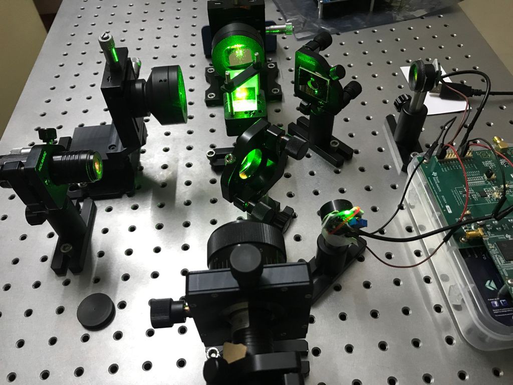
Seeing the distinct interference fringes from the green measurement laser and the red reference laser provides immediate visual proof of the system's ability to monitor both wavelengths simultaneously

Michelson Interferometer with Green Laser 

Michelson Interferometer with Red Laser 

The Heart of the Rings: How It Works

The magic of the circular fringes is rooted in the precision of the interferometer's setup.

1. Splitting the Beam: The red laser light, typically from a Helium-Neon (He-Ne) laser with a wavelength (λ) around 632.8 nm, hits a beam splitter. This semi-silvered mirror divides the single beam into two coherent beams: one reflected and one transmitted.
2. Path Difference: These two beams travel along perpendicular paths, reflect off two separate mirrors (M1 and M2), and then return to recombine at the beam splitter. The resulting pattern depends on the optical path difference ($\Delta x$) between the two arms of the interferometer.
3. Achieving the Rings: To get circular fringes, the two mirrors (M1 and M2's virtual image) must be set up to be perfectly perpendicular to each other, or as close as possible. This creates an effect where the path difference, Δx, depends only on the angle of inclination ($\theta$) at which the light rays leave the extended laser source (which is typically broadened by a lens).

The Mathematics of the Rings

The conditions for the interference pattern are:

Bright Fringes (Constructive Interference):

where is the effective distance between the two mirrors, is the angle of inclination, and is an integer known as the order of the fringe.

Dark Fringes (Destructive Interference):

Since , (the red light's wavelength), and are constant for a specific ring, the angle is also constant. All points on the screen that correspond to the same angle of inclination will have the same path difference and therefore the same intensity, forming a perfect circle centered on the optical axis. These are often called fringes of equal inclination.

Watching the Rings Breathe

One of the most exciting parts of the experiment is observing the movement of the fringes as you carefully adjust the movable mirror, .

• Mirror Movement: When M1 is moved slightly, the distance changes. According to the equation, 2dcosθ=mλ , this changes the order for a given angle .
• Shrinking and Expanding: If you slowly move a mirror to decrease the path difference d , you will see the circular fringes shrink and disappear at the center. If you increase d, new fringes appear at the center and expand outward.

By counting the number of red fringes (N) that pass a fixed point as the mirror is moved a known distance (Δd), you can precisely determine the red laser's wavelength using the relationship:

The circular fringes of a red laser in a Michelson interferometer are not just a beautiful sight—they are a powerful, tangible tool used in science and engineering to make incredibly precise measurements of distance, wavelength, and refractive index.

In the precise world of Fourier-transform infrared (FTIR) spectroscopy, the integrity of the optical path is paramount. Two fundamental optical components often used for beam steering are the plane mirror and the retro-reflector, also known as a corner cube prism. While both serve to redirect light, their operating principles and performance differ dramatically, with a key figure of merit—beam deviation—determining their suitability for the demanding application of an FTIR interferometer.

Beam deviation is the angular change in the direction of a light beam after it is reflected. In an FTIR, a delicate interference pattern is created by combining a beam that has travelled a fixed distance with one from a moving mirror. This requires the beams to remain perfectly aligned and overlapped at the detector. Even a minute beam deviation would cause the return beam to fail to overlap with the static beam, leading to a reduction in the interference signal and, in the worst case, a complete loss of signal, resulting in a distorted or non-existent spectrum.

The Plane Mirror: A Foundation of Reflection

A plane mirror is a simple, flat surface that reflects light according to the law of reflection: the angle of incidence (θi) equals the angle of reflection (θr). This straightforward relationship makes it ideal for basic beam steering or folding the optical path in a fixed optical setup.

The primary disadvantage of a plane mirror is its extreme sensitivity to alignment. Any angular misalignment or tilt (α) of the mirror surface results in a doubling of the beam deviation to 2α. To put this into perspective, for a light beam traveling a meter to a mirror and back, a misalignment of just 0.1∘ would cause the returning beam to shift by over 3.4 millimeters. For the dynamic movement required in an FTIR, this sensitivity makes a plane mirror impractical. The mechanical precision needed to keep a moving mirror perfectly parallel to the beamsplitter is virtually impossible to achieve, causing the return beam to wander and miss the detector entirely.

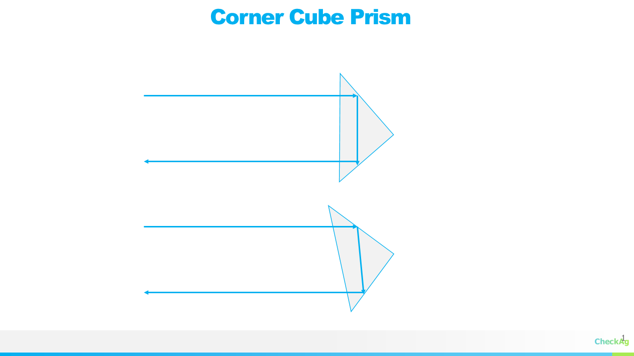
The Retro-reflector: The Ultimate in Beam Stability

A retro-reflector is an optical component designed to reflect an incident light beam back along a path that is precisely parallel to the incoming beam, regardless of the angle of incidence. The most common type is a corner cube prism, which consists of three mutually perpendicular reflecting surfaces. This ingenious geometry ensures the output beam's direction is always corrected.

The operating principle relies on a series of three sequential reflections. As the incoming ray hits each of the three mutually perpendicular surfaces, its vector components are successively reversed. This triple-reflection geometry ensures the emergent ray is anti-parallel to the incident ray, making the output beam precisely parallel to the input. This property holds true even if the entire prism is slightly tilted or misaligned, as the corrections from the three reflections cancel out the initial misalignment. This allows for a very high tolerance for alignment errors.

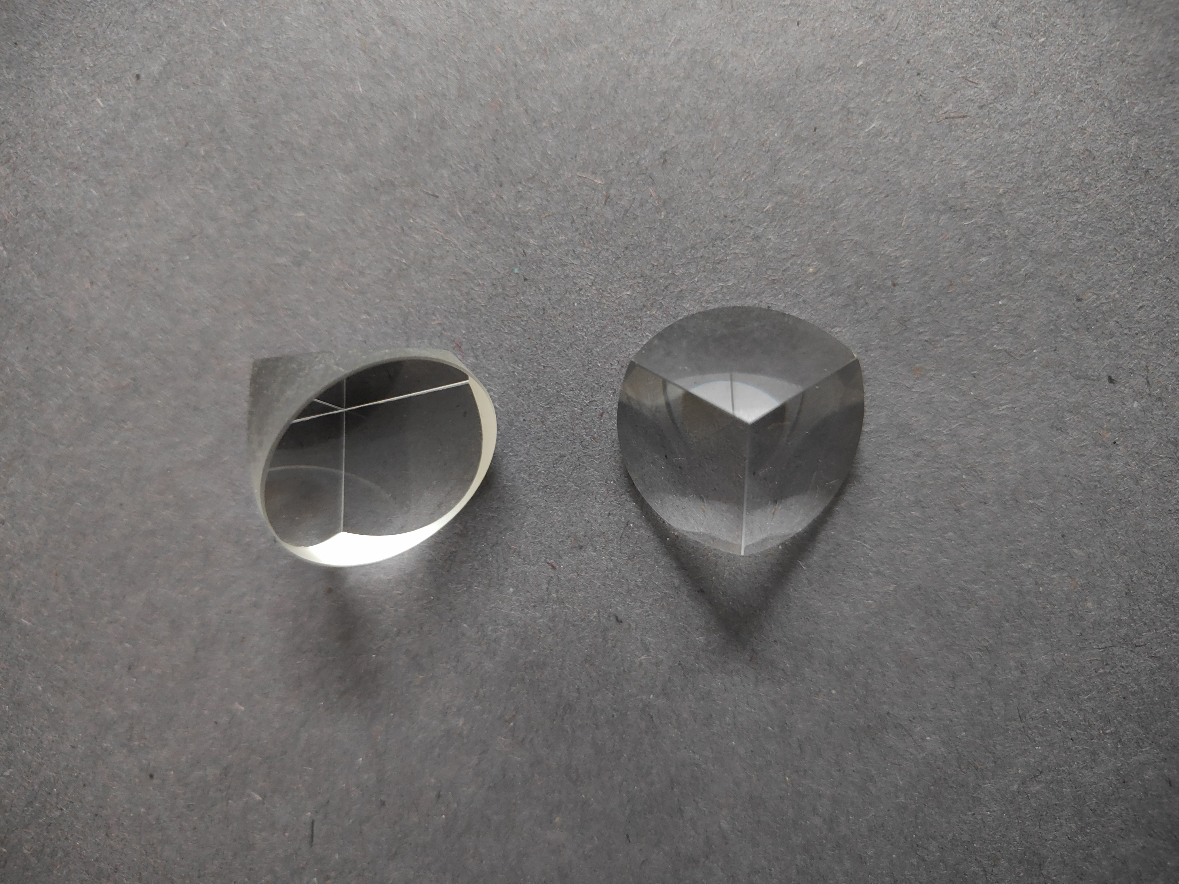
A Note on Retro-reflector Materials

The solid retro-reflector prisms, often made from materials like BK-7 glass, are indeed used for white light interferometry. The reason for this is practical: it is much easier to view and align white light fringes with visible light. For this purpose, a solid prism is a simple and effective choice. However, these prisms are not transparent to infrared (IR) light. Because the light source in an FTIR is in the infrared range, a solid glass prism would simply absorb the beam, making it useless for the spectrometer. For this reason, FTIR instruments rely on hollow retro-reflector mirrors, which are constructed from three flat mirrors arranged in a corner cube configuration. This design provides the same self-correcting optical path without the need for a solid, absorbing material in the beam path.

Comparison and Application in FTIR

The contrast between these two components makes the choice for an FTIR interferometer clear. The moving mirror must maintain perfect parallelism to ensure the recombining beams create a stable interferogram. A plane mirror would require impossible mechanical precision, as the moving stage would have to be perfectly straight and level across its entire range of motion. The retro-reflector, however, can handle the minute mechanical imperfections of the moving stage, automatically correcting the beam's path and ensuring it consistently returns to the beamsplitter. 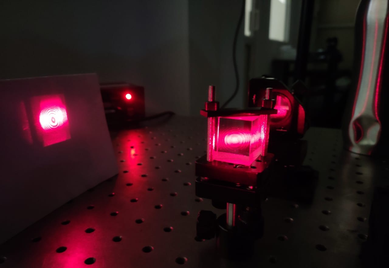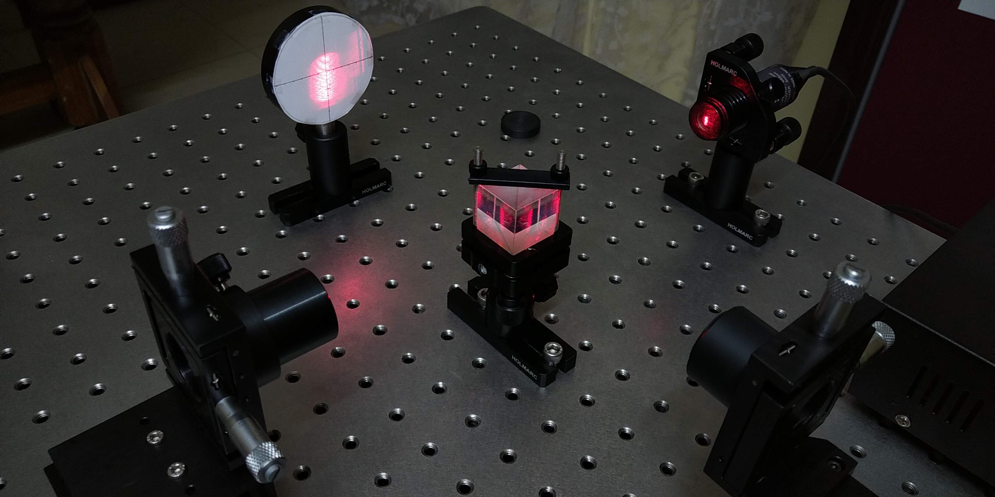This inherent stability is why retro-reflectors are the standard in modern FTIR instruments, as they enable the robust, continuous-scanning performance needed for accurate and reproducible measurements, even in dynamic or vibration-prone environments.

The initial setup for our Michelson interferometer is complete. We've chosen to use retroreflector mirrors for the setup, a design choice critical for both Fourier Transform Infrared (FTIR) spectroscopy and our current visible-light testing.

In our setup, the two retroreflector mirrors are mounted on linear stages, which allow us to precisely control their displacement. These stages facilitate the movement of one mirror relative to the other, creating a variable optical path difference (OPD). The heart of the interferometer is the cube beamsplitter, which divides the incoming light beam into two paths and then recombines them after reflection from the mirrors. Because the beamsplitter is a cube, both paths traverse the same amount of glass, inherently providing an equal path length and eliminating the need for a separate compensation plate.

The interferogram, which is the raw interference pattern, is then captured on a screen. The appearance of circular fringes in the interferogram is a key indicator of proper alignment. These fringes arise from the interference of wavefronts with a slight difference in their angle of incidence, signifying that the mirrors are well-aligned and the optical system has a near-perfect geometry.

Next Steps

Moving forward, our next step is to design and implement a detector circuit to electronically capture the interferogram. We will also publish a detailed note explaining the importance and functionality of retroreflectors in interferometry, highlighting why they are superior to plain mirrors for applications requiring high precision.

As part of our ongoing efforts to make complex optical principles more accessible, we've prepared an Octave script that beautifully illustrates the concepts of signal interference and Fast Fourier Transform (FFT), which are fundamental to how FTIR spectrometers work.

You can find our latest log post, "Unveiling the Spectrum: Demystifying Interference with FFT," on Hackaday here: https://hackaday.io/project/202423-jasper-ftir/log/242500-unveiling-the-spectrum-demystifying-interference-with-fft. The post features two aspects 

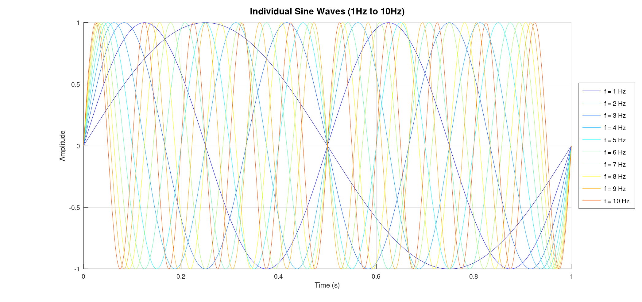
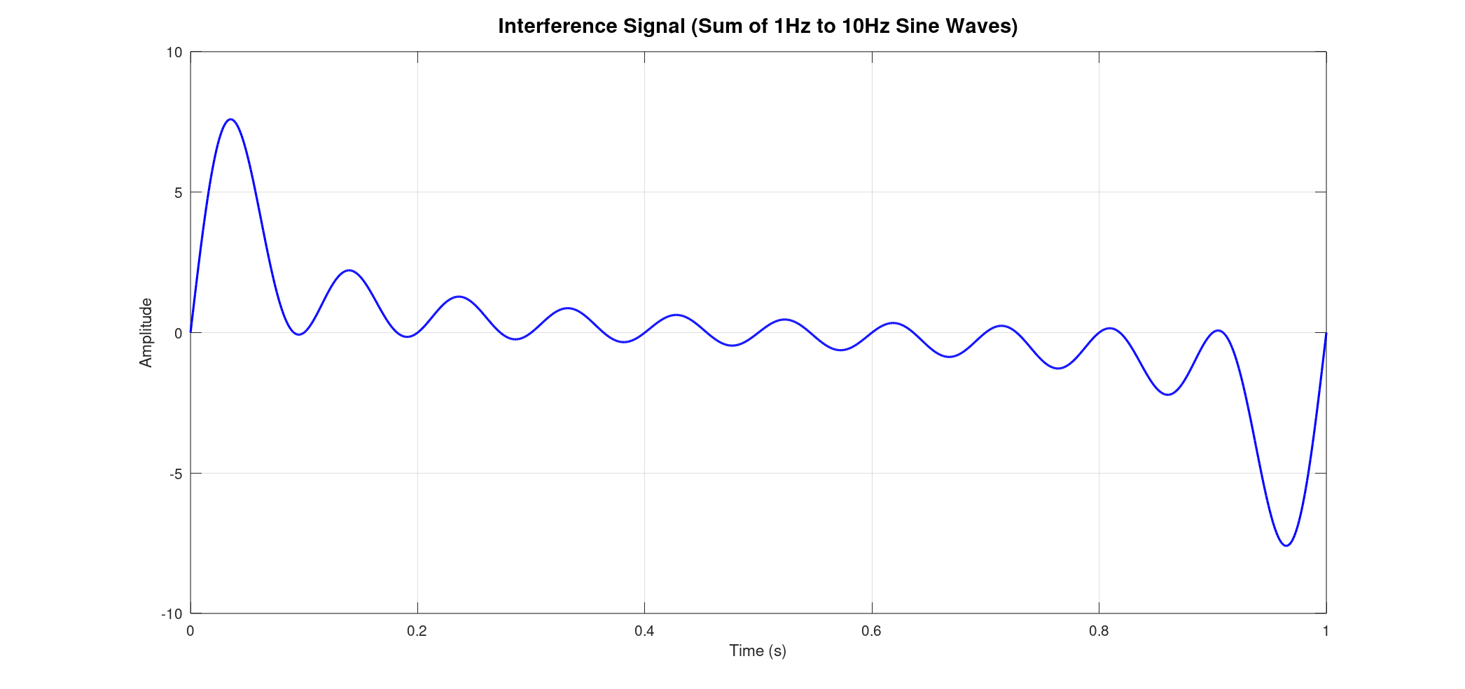
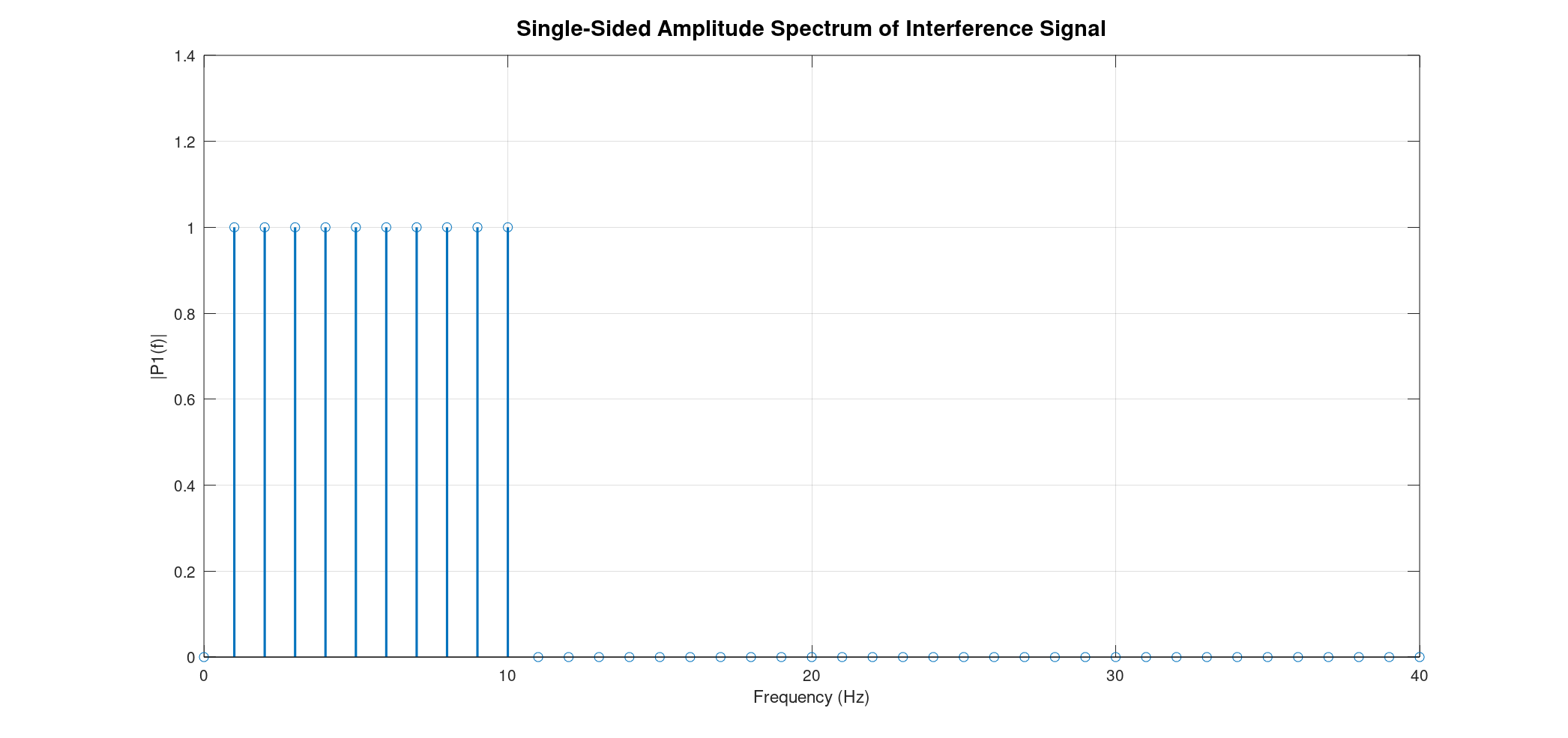
1. Uniform Intensity Sine Waves: We generate a series of sine waves, all with the same intensity, ranging from 1 Hz to 10 Hz. You'll see these individual waves plotted, followed by their combined interference pattern. Crucially, the FFT of this combined signal will show distinct peaks at each of the original frequencies, all with uniform intensity, demonstrating how FFT can decompose a complex signal into its constituent frequencies.
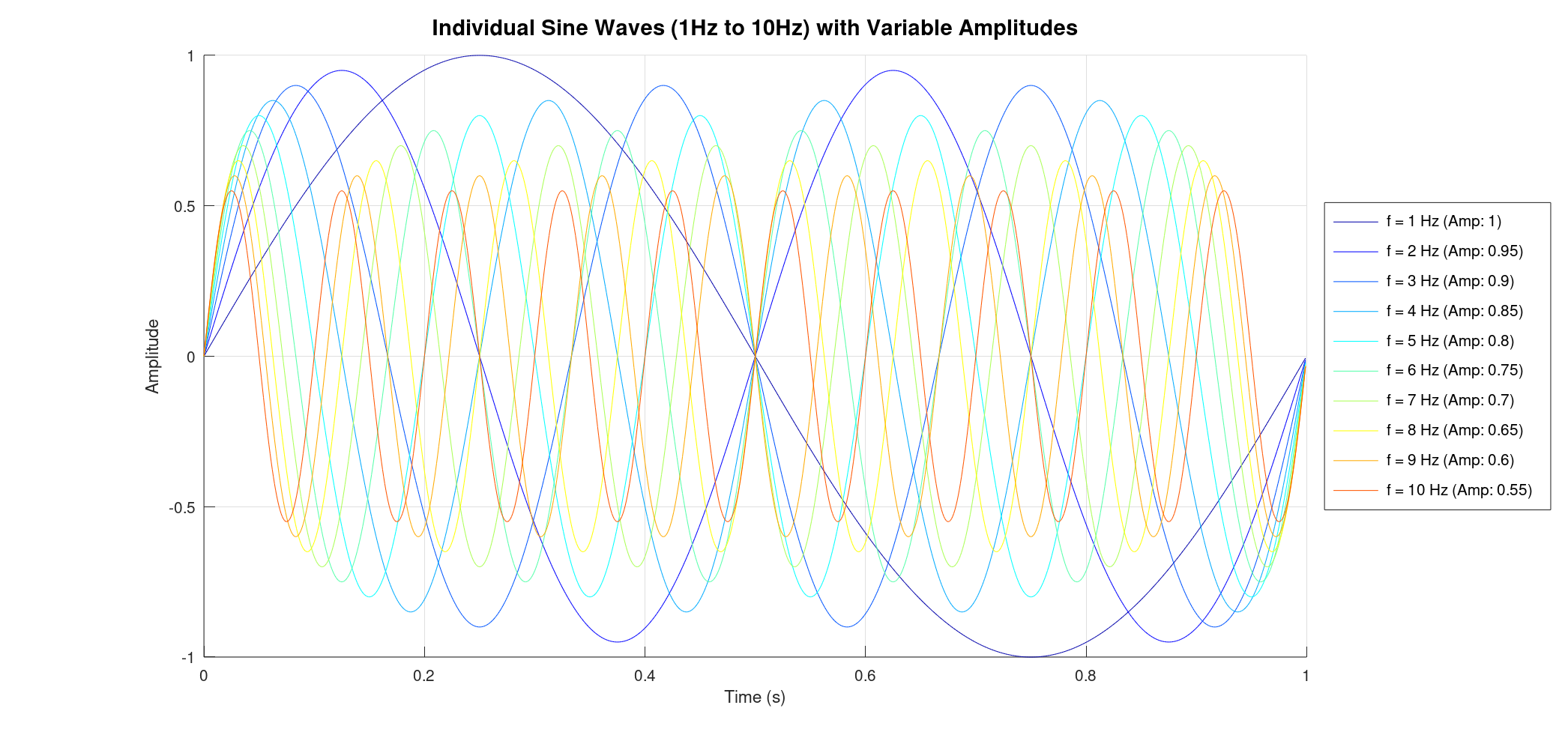
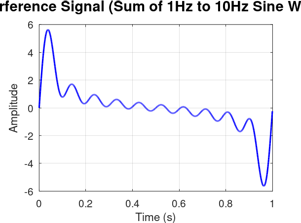
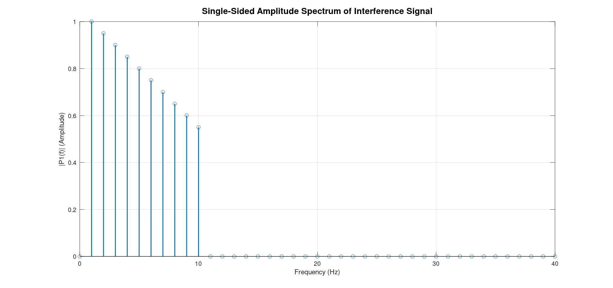
2. Variable Intensity Sine Waves: In this section, we repeat the process, but this time, the sine waves have varying intensities. This simulates a more realistic scenario where different frequencies might have different strengths. Again, we plot the individual waves, their interference, and then their FFT. The FFT in this case will reveal peaks at the original frequencies, but their heights will correspond to the varying intensities, providing insight into the spectral content of the signal.

All the illustrations and plots in the Hackaday post were generated using this Octave code.

We will be setting up a git hub repository where the code will be uploaded. But for now, check the code here 

We encourage you to run this code, experiment with the parameters, and see the magic of Fourier Transform in action. Your feedback and contributions are always welcome as we continue to build JASPER FTIR together!

% --- Parameters for Sine Wave Generation ---
f_min = 1;          % Minimum frequency of sine waves (Hz)
f_max = 10;         % Maximum frequency of sine waves (Hz)
overSampRate = 100; % Oversampling rate (samples per highest frequency cycle)
nCyl = 1;           % Number of cycles for the lowest frequency (f_min) to display

% Define variable amplitudes for each sine wave
% This array should have 'f_max - f_min + 1' elements
% Example: decreasing amplitude with increasing frequency
amplitudes = [1.0, 0.95, 0.9, 0.85, 0.8, 0.75, 0.7, 0.65, 0.6, 0.55];
% Ensure the number of amplitudes matches the number of frequencies
if length(amplitudes) ~= (f_max - f_min + 1)
    error('The number of amplitudes must match the number of frequencies (f_max - f_min + 1).');
end

% --- Derived Parameters for Time Domain ---
% Sampling frequency must be high enough to accurately represent the highest frequency
fs = overSampRate * f_max;
% Time base: spans 'nCyl' cycles of the lowest frequency (f_min)
% Adjusted time vector to ensure signal length aligns perfectly with integer frequency bins
t = 0 : 1/fs : (nCyl * 1/f_min - 1/fs); % Ensure L = fs * duration for exact bin alignment

% --- Generate and Plot Individual Sine Waves ---
figure(1);
hold on; % Keep all plots on the same figure
all_sine_waves = zeros(length(t), f_max - f_min + 1); % Pre-allocate matrix for all sine waves
legend_entries = cell(1, f_max - f_min + 1); % Pre-allocate cell array for legend entries

% Generate a colormap for distinct colors for each sine wave
colors = jet(f_max); % 'jet' colormap provides a good range of colors

fprintf('Generating and plotting individual sine waves...\n');
for k = f_min : f_max
    current_amplitude_idx = k - f_min + 1;
    current_amplitude = amplitudes(current_amplitude_idx);

    % Generate sine wave for current frequency k with its specific amplitude. Phase is 0.
    y = current_amplitude * sin(2 * pi * k * t);

    % Store the sine wave for later summation
    all_sine_waves(:, current_amplitude_idx) = y;

    % Plot the individual sine wave with a unique color from the colormap
    plot(t, y, 'color', colors(k,:), 'DisplayName', ['f = ', num2str(k), ' Hz, Amp = ', num2str(current_amplitude)]);

    % Store legend entry
    legend_entries{current_amplitude_idx} = ['f = ', num2str(k), ' Hz (Amp: ', num2str(current_amplitude), ')'];
end

% Add title and labels for the individual waves plot
title(['Individual Sine Waves (', num2str(f_min), 'Hz to ', num2str(f_max), 'Hz) with Variable Amplitudes'],'FontSize', 14);
xlabel('Time (s)');
ylabel('Amplitude');
% Display legend outside the plot area for better visibility
legend(legend_entries, 'Location', 'eastoutside', 'FontSize', 10);
grid on; % Add a grid for better readability
hold off; % Release the hold on the figure

% --- Generate and Plot Interference Signal ---
% Sum all the individual sine waves to get the interference signal
interference_signal = sum(all_sine_waves, 2);

figure(2);
% Plot the interference signal in blue with a slightly thicker line
plot(t, interference_signal, 'b', 'LineWidth', 1.5);
title(['Interference Signal (Sum of ', num2str(f_min),'Hz to ', num2str(f_max), 'Hz Sine Waves)'],'FontSize', 14);
xlabel('Time (s)');
ylabel('Amplitude');
grid on; % Add a grid for better readability

fprintf('Done with time domain plots.\n');

% --- Fast Fourier Transform (FFT) Analysis ---

% Parameters for FFT, derived from time domain parameters
Fs_fft = fs;                 % Sampling frequency for FFT (Hz)
L = length(interference_signal); % Length of the signal
T_fft = 1/Fs_fft;            % Sampling period

% Perform FFT on the interference signal
Y = fft(interference_signal);

% --- Plotting FFT Results ---

% Figure 5: Single-Sided Amplitude Spectrum
P2 = abs(Y/L);
P1 = P2(1:L/2+1);
P1(2:end-1) = 2*P1(2:end-1); % Multiply by 2 for positive frequencies (except DC and Nyquist)

figure(3); % Renamed from figure(5) as figure 3 and 4 are removed
f_plot = Fs_fft/L*(0:(L/2));
% Changed plot to stem to show distinct frequency lines
stem(f_plot, P1, "LineWidth", 1.5);
title("Single-Sided Amplitude Spectrum of Interference Signal", "FontSize", 14);
xlabel("Frequency (Hz)");
ylabel("|P1(f)| (Amplitude)");
xlim([0 f_max + 30]); % Set x-axis limit as requested
grid on;

fprintf('Done with FFT plots.\n');

In our last post, we explored how simple sine waves can combine to create complex interference patterns, and we briefly touched upon the magic of the Inverse Fast Fourier Transform (IFFT) to reconstruct a signal from its frequency components. Today, we're flipping the script! We'll dive deeper into the Fast Fourier Transform (FFT) to see how it allows us to dissect a complex interference signal and reveal its constituent frequencies and their individual strengths. Think of it as a powerful lens that transforms a jumbled waveform into a clear "fingerprint" of its underlying vibrations.

Part 1: The Symphony of Uniform Amplitudes 🎶

Let's start with a foundational example. Imagine we have ten pure sine waves, ranging in frequency from 1 Hz to 10 Hz. Crucially, each of these waves has the exact same amplitude (intensity).

When these ten waves combine, they create a fascinating, yet seemingly chaotic, interference pattern. This resulting signal is the sum of all individual waves, oscillating in a complex dance.

Now, for the big reveal! When we apply the FFT to this interference signal, the results are remarkably clear. The FFT transforms the signal from the time domain (how amplitude changes over time) to the frequency domain (what frequencies are present and how strong they are). What we see is a series of 10 distinct vertical lines at precisely 1 Hz, 2 Hz, 3 Hz, and so on, up to 10 Hz. The height of each line directly corresponds to the amplitude of that specific sine wave in the original signal. Since all our initial sine waves had uniform amplitudes, all these lines in the FFT plot will have the same height, beautifully demonstrating their equal contribution to the interference.

Part 2: Decoding Variable Intensities with FFT 

The real power of FFT shines when the individual components of our signal aren't so uniform. What if each of our 1 Hz to 10 Hz sine waves had a different amplitude? For instance, the 1 Hz wave might be very strong, while the 10 Hz wave is much weaker.

When these variable-amplitude waves interfere, the resulting signal still looks complex, but its shape is now influenced more heavily by the stronger frequency components.

Applying the FFT to this new interference signal is where it gets truly exciting! Just like before, we'll see distinct lines at each frequency (1 Hz to 10 Hz). However, this time, the height of each line will vary, directly reflecting the unique amplitude of each sine wave in the original mix. This is incredibly powerful! In applications like spectroscopy, this varying amplitude in the frequency domain is analogous to absorbance levels, where the intensity of a peak tells us how much of a particular substance is present or how strongly it interacts at that specific frequency. The FFT allows us to quantify these "absorbance levels" without needing to isolate each individual wave.

The Fast Fourier Transform is an indispensable tool in signal processing, allowing us to decompose complex time-domain signals into their fundamental frequency components. Whether the amplitudes are uniform or varying, the FFT provides a clear and quantitative representation of the spectrum, making it invaluable for everything from audio analysis to scientific measurements where understanding "absorbance" or signal strength at specific frequencies is key. 

This principle is at the heart of techniques like Fourier-Transform Infrared (FTIR) Spectroscopy. In FTIR, an interferometer creates an interferogram (much like our interference signal), which is a time-domain representation of how a sample absorbs different infrared wavelengths. The raw interferogram is then fed into an FFT algorithm, which transforms it into an infrared spectrum. This spectrum reveals distinct peaks at specific infrared frequencies, and the intensity (or "absorbance") of these peaks directly corresponds to the unique vibrational modes of the molecules within the sample, allowing for precise chemical identification and quantification. Our simple sine wave example beautifully illustrates the fundamental mathematical operation that underpins this powerful analytical technique.

Have you ever wondered how scientists analyze the chemical composition of materials without destroying them? One powerful technique is Fourier Transform Infrared (FTIR) Spectroscopy, and at its heart lies a fascinating principle: wave interference.

Let's break down how simple sine waves, when combined, can lead us to understand the complex signals measured by an FTIR spectrometer.

The Dance of Simple Waves: Interference Basics

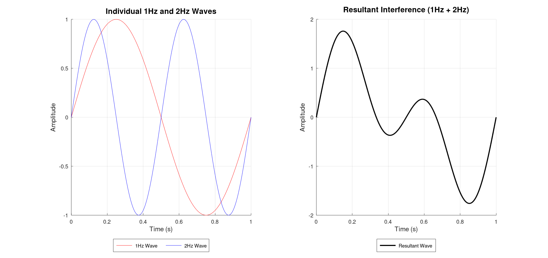
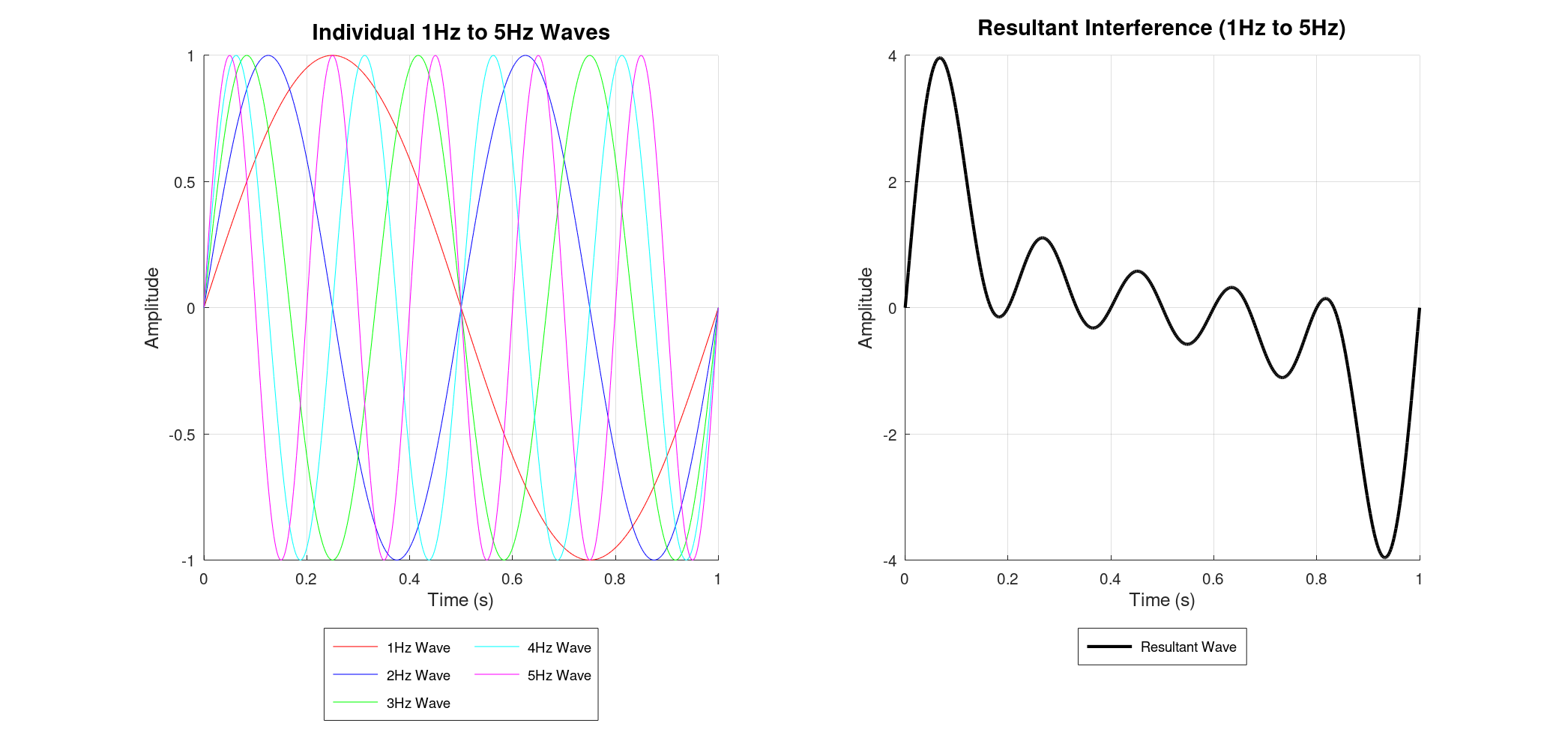
Imagine two simple sine waves, one at 1 Hz and another at 2 Hz. When these waves travel through the same space, they interact, or "interfere." This interference is simply the sum of their amplitudes at every point in time.

If you were to plot these individual waves and then their sum, you'd see how their peaks and troughs align (constructive interference) or cancel out (destructive interference), creating a new, more complex waveform.

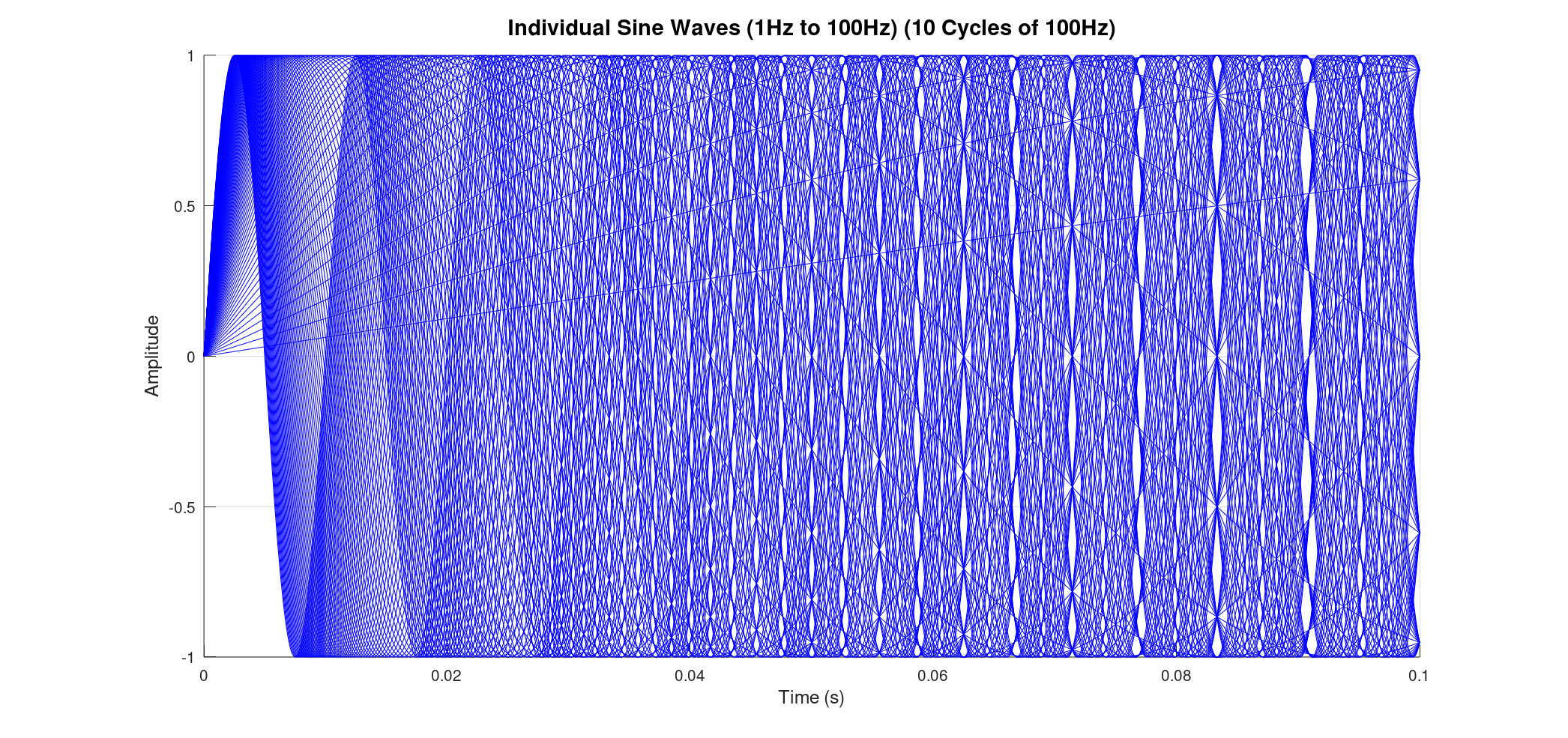
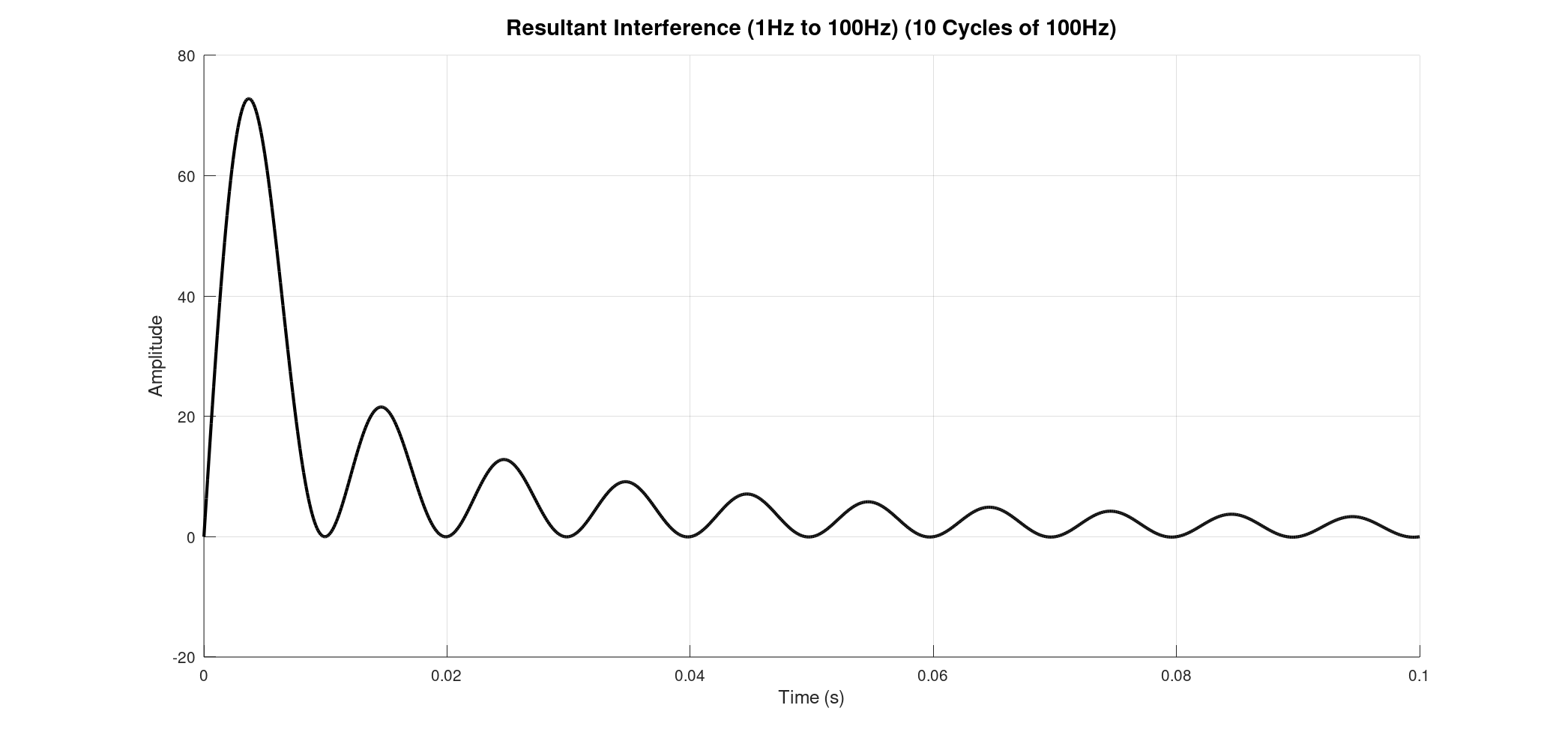
As we add more and more sine waves – say, from 1 Hz up to 5 Hz and even 1 Hz to 100 Hz – the resultant waveform becomes progressively more intricate. Each additional frequency contributes its unique oscillation, making the combined signal look less like a simple wave and more like a chaotic squiggle.

Building Complexity: From Many Waves to a "Fingerprint"

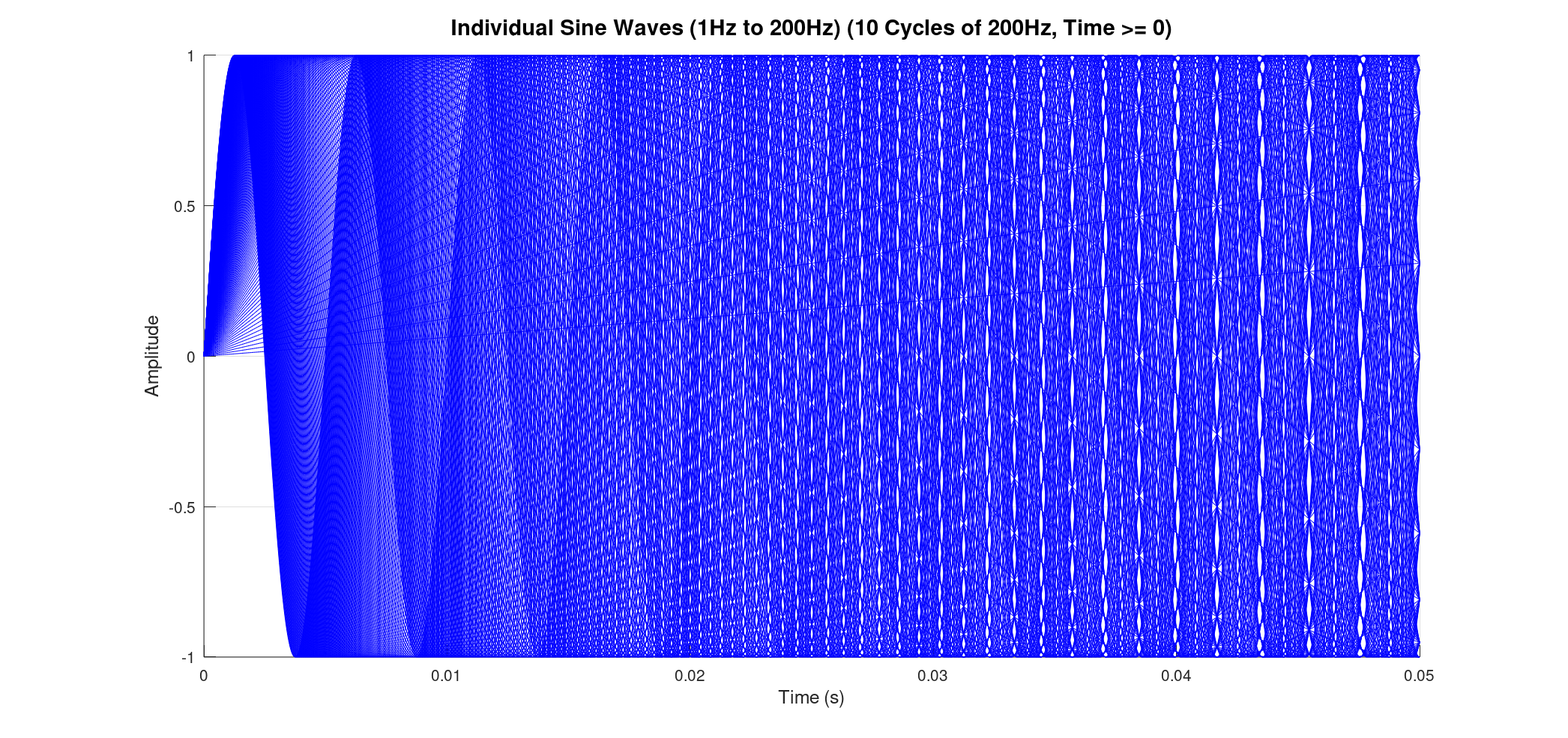
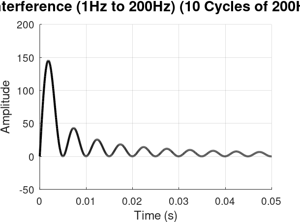
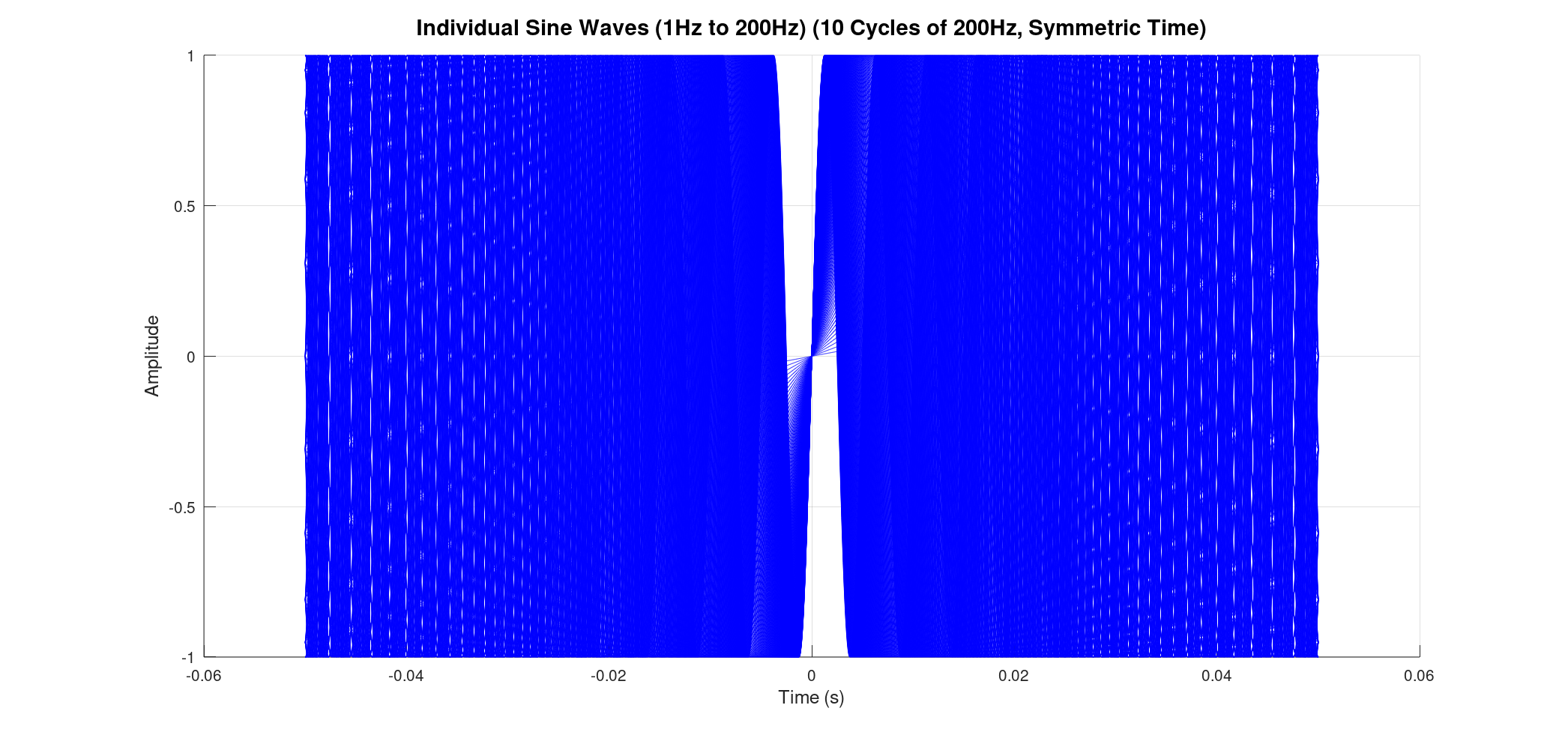
Consider summing a vast number of sine waves, from 1 Hz all the way up to 200 Hz, each at 1 Hz intervals. When we plot all these individual waves, they appear as a dense, almost solid band of blue lines, showcasing the sheer volume of oscillations contributing to the final signal. The resultant sum, while still a single black line, is now incredibly complex, reflecting the combined energy of all those frequencies.

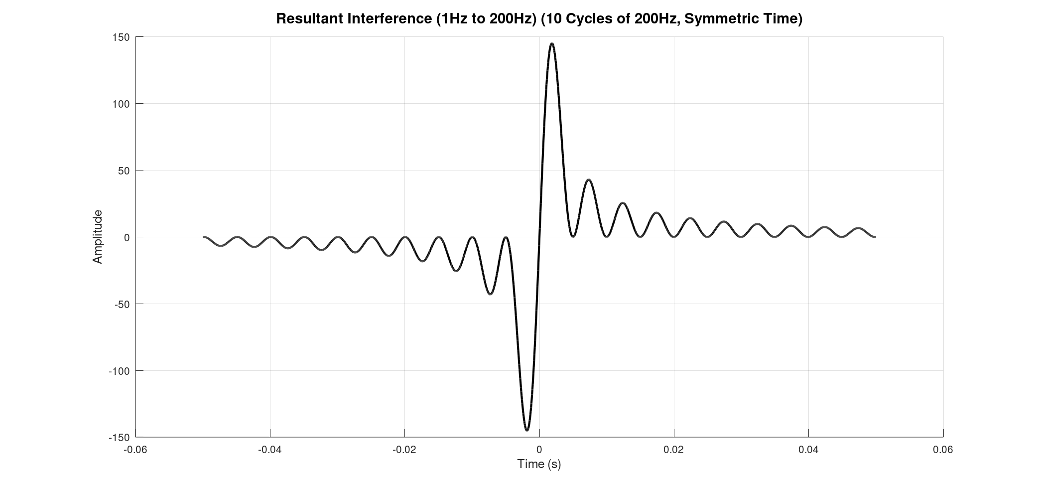
Previously, we might have plotted these waves starting from time zero and extending for a certain duration. However, for FTIR, a symmetric time base is essential. This means our time axis extends from a negative value, passes through zero, and continues to a positive value (e.g., from -0.05 seconds to +0.05 seconds for our 1-200Hz example, based on 10 cycles of the 200Hz wave).

Why symmetric? This directly relates to the core of an FTIR spectrometer: the Michelson interferometer. In this device, a beam of light is split, travels different path lengths, and then recombines. The "time" axis in our plots is analogous to the optical path difference (OPD) between the two arms of the interferometer.

Zero Path Difference (ZPD). At this point, all the individual waves, regardless of their frequency, are perfectly in phase and constructively interfere. This creates a very strong, central peak in the resultant interference signal. As the optical path difference moves away from zero (either positively or negatively), the waves start to fall out of phase, leading to destructive interference and a rapid decrease in the signal's intensity. This unique signal, with its prominent central peak and decaying oscillations, is what we call an interferogram

From Interferogram to Spectrum: The Power of Fourier Transform 

The magic of FTIR lies in its ability to convert this complex interferogram into a chemically meaningful spectrum. This transformation is achieved using a mathematical tool called the Fourier Transform (FT).

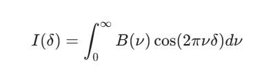
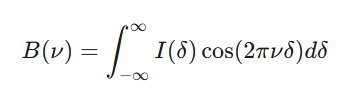
Imagine our interferogram, , as a function of the optical path difference, $\delta$. This interferogram is essentially the sum of many individual cosine waves, each corresponding to a specific frequency of light that passed through the sample. A simplified representation could be:

Where:

• is the intensity of the interferogram at a given optical path difference $\delta$.
• $B(\nu )$ is the spectral intensity at wavenumber $\nu$ (which is directly related to frequency).
• $\cos (2\pi \nu \delta )$ represents the individual cosine waves that sum up.

To get the spectrum, $B(\nu )$, from the interferogram, $I(\delta )$, we perform the inverse Fourier Transform:

In practice, a fast Fourier transform (FFT) algorithm is used by the spectrometer's computer to perform this calculation. The result is a plot of intensity (or absorbance/transmittance) versus wavenumber (or frequency), which is the characteristic spectrum of your sample. This spectrum acts like a unique "fingerprint," allowing scientists to identify and quantify the chemical components present in a material.

By understanding how simple waves combine and how the time base in our plots mirrors the optical path difference in an interferometer, we can grasp the fundamental principles that make FTIR spectroscopy such a powerful analytical technique.

Our first step in developing the JASPER FTIR spectrometer is to master the core component: the Michelson interferometer. To begin, we are building a setup using a red diode laser. While a He-Ne laser is a common choice, our long-term goal is to use a ZnSe beamsplitter instead of the hygroscopic KBr. Since ZnSe is not transparent in the visible range where the He-Ne spectrum lies, a red diode laser is a more suitable choice for our initial prototype.

We're using a cube beamsplitter, which simplifies the design by ensuring equal path lengths for the two optical arms. This eliminates the need for a compensating optical window, making our initial implementation significantly easier.

The interference fringes from the red diode laser will be observed on a ground glass screen. We'll start with flat mirrors to achieve our first fringes and later transition to retroreflectors. We are still researching the accuracy requirements for retroreflectors and their limitations in this application.

To validate our components, particularly the retroreflectors and the cube beamsplitter, we've had to take a leap of faith and order them without a clear validation plan. We'll be holding our breath until we have the setup running to see if we can achieve those coveted white light interference fringes. Follow along as we learn, iterate, and (hopefully) succeed!

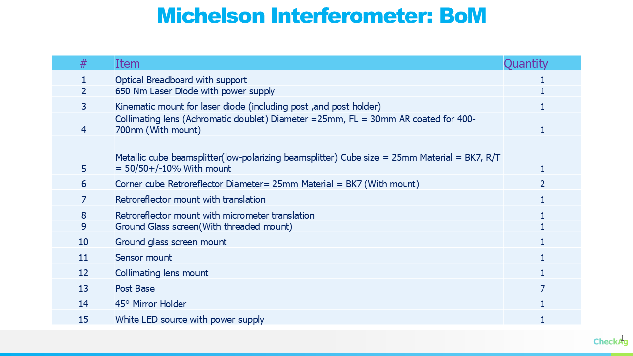
Bill of Materials for the Michelson Interferometer: 

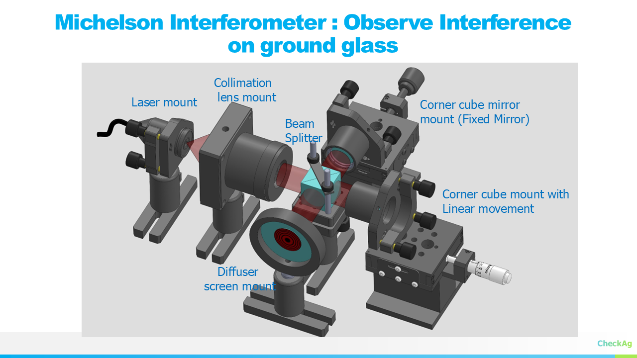
3D Visualization of the Setup: